Chapter 2 Prepare and Describe the Data

This chapter prepares the data set and does some univariate and multivariate description of its characteristics prior to the CFA implementation in later chapters. Both numeric and graphical description and inference about distribution shape are quickly available with R functions from the psych and MVN packages.

2.1 The Data Set

The 175 case data set (no missing observations) is loaded from a .csv file. The .csv file was exported from the SPSS system file that is available from the website for the Tabachnick textbook (Tabachnick et al., 2019) It has eleven subscales from the WISC:

info (Information)
comp (Comprehension)
arith (Arithmetic)
simil (Similarities)
vocab (Vocabulary)
digit (Digit Span)
pictcomp (Picture Completion)
parang (Picture Arrangement)
block (Block Design)
object(Object Assembly)
coding (Coding - not sure if it is A or B, or a combination)

The user may recognize these scales as commonly discussed subtests of the WISC. The first 6 variables comprise the set of manifest variables for the latent factor known as Verbal. The last five are associated with Performance.

The original data file also contains an ID variable that is dropped for the working object created as wisc2 here.

# import the primary data file
wisc1 <- read.csv("wisc1.csv")
knitr::kable(head(wisc1),booktabs=TRUE,format="markdown")

ID	info	comp	arith	simil	vocab	digit	pictcomp	parang	block	object	coding
3	8	7	13	9	12	9	6	11	12	7	9
4	9	6	8	7	11	12	6	8	7	12	14
5	13	18	11	16	15	6	18	8	11	12	9
6	8	11	6	12	9	7	13	4	7	12	11
7	10	3	8	9	12	9	7	7	11	4	10
8	11	7	15	12	10	12	6	12	10	5	10

# create the working data frame by removing the ID variable
wisc2 <- wisc1[,2:12]

A note about tables in this document: Many of the tables generated by the various R functions in this document are reformatted so that they do not appear as the plain text that is typically output into the R console. The kable function in the knitr package permits formatting that is well-rendered with rmarkdown and bookdown document production. kable is used frequently.

2.2 Numeric and Graphical Description of the Data

We can explore univariate characteristics of the data with summaries, plots, and evaluation of normality characteristics

2.2.1 Univariate descriptive statistics from the psych package.

knitr::kable(describe(wisc2,type=2,fast=T),booktabs=TRUE,format="markdown")

	vars	n	mean	sd	min	max	range	se
info	1	175	9.497143	2.912269	3	19	16	0.2201469
comp	2	175	10.000000	2.965317	0	18	18	0.2241569
arith	3	175	9.000000	2.306911	4	16	12	0.1743861
simil	4	175	10.611429	3.183630	2	18	16	0.2406598
vocab	5	175	10.702857	2.932721	2	19	17	0.2216929
digit	6	175	8.731429	2.704166	0	16	16	0.2044157
pictcomp	7	175	10.680000	2.934221	2	19	17	0.2218063
parang	8	175	10.371429	2.659679	2	17	15	0.2010528
block	9	175	10.314286	2.709831	2	18	16	0.2048440
object	10	175	10.902857	2.843978	3	19	16	0.2149845
coding	11	175	8.548571	2.872118	0	15	15	0.2171117

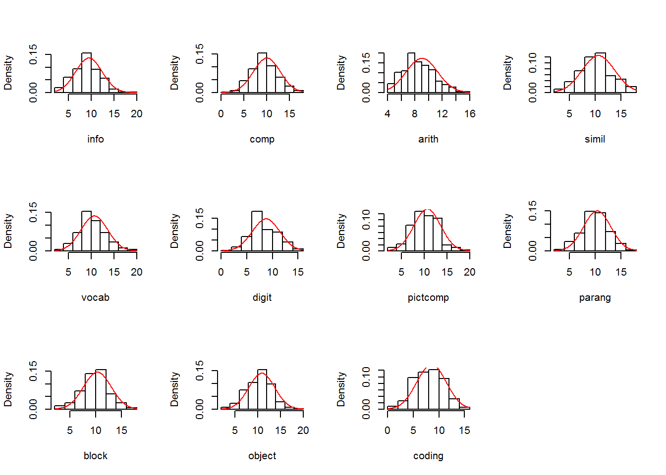
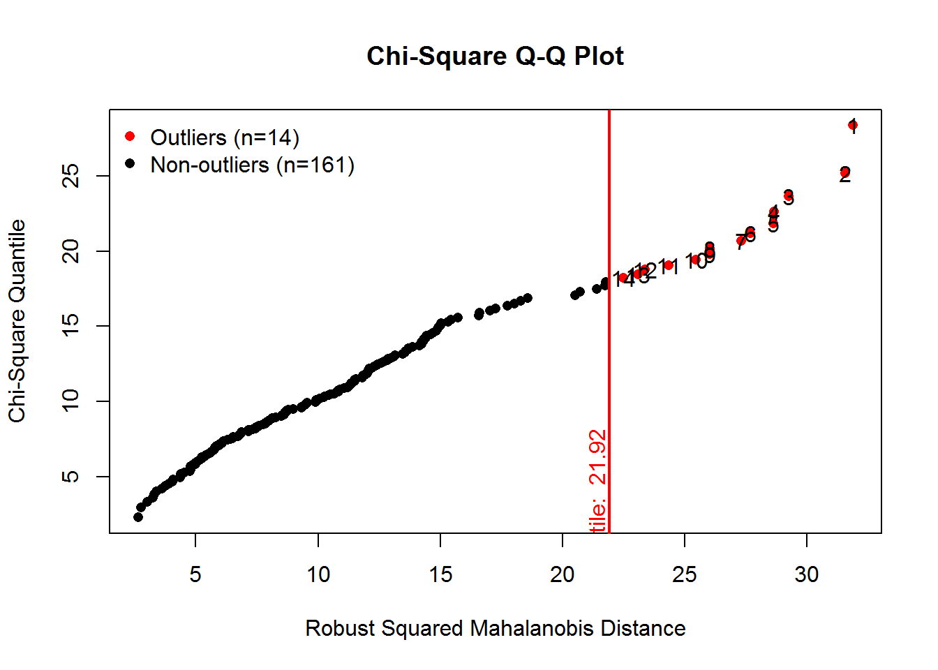
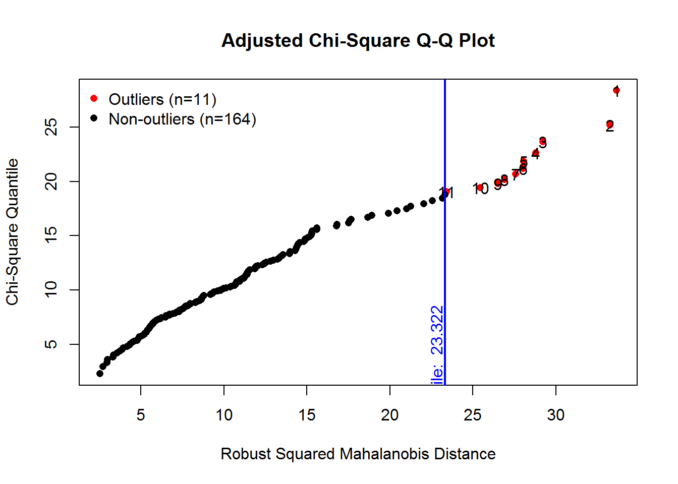
2.2.2 Univariate Distribution Tests and Plots plus Evaluation of Multivariate Normality

The MVN package provides univariate and multivariate normality tests. It is an efficient way to explore characteristics of a set of variables. Several options are available for testing both univariate and Multivariate normality. First, explicit calls for univariate and multivariate tests are made, and then an approach is shown that obtains all at once plus a useful set of plots.

x_vars <- wisc2
# use the mvn function for an extensive evaluation
# note that different kinds of tests can be specified with changes in the arguments
result <- mvn(data= x_vars, mvnTest="mardia",  univariateTest="AD")
kable(result$univariateNormality, booktabs=TRUE, format="markdown")

Test	Variable	Statistic	p value	Normality
Anderson-Darling	info	1.2049	0.0037	NO
Anderson-Darling	comp	1.3546	0.0016	NO
Anderson-Darling	arith	1.8656	1e-04	NO
Anderson-Darling	simil	0.9336	0.0175	NO
Anderson-Darling	vocab	1.4992	7e-04	NO
Anderson-Darling	digit	2.5087	<0.001	NO
Anderson-Darling	pictcomp	1.1472	0.0052	NO
Anderson-Darling	parang	1.3391	0.0017	NO
Anderson-Darling	block	1.5225	6e-04	NO
Anderson-Darling	object	1.1593	0.0049	NO
Anderson-Darling	coding	1.2217	0.0034	NO

kable(result$multivariateNormality, booktabs=TRUE, format="markdown")

Test	Statistic	p value	Result
Mardia Skewness	348.496907430775	0.00673137335852766	NO
Mardia Kurtosis	2.30789388829536	0.0210050390817529	NO
MVN	NA	NA	NO

kable(mvn(data= x_vars,univariatePlot="histogram"), booktabs=TRUE, format="markdown")

Test	Statistic	p value	Result
Mardia Skewness	348.496907430775	0.00673137335852766	NO
Mardia Kurtosis	2.30789388829536	0.0210050390817529	NO
MVN	NA	NA	NO

Test	Variable	Statistic	p value	Normality
Shapiro-Wilk	info	0.9814	0.0194	NO
Shapiro-Wilk	comp	0.9810	0.0170	NO
Shapiro-Wilk	arith	0.9709	0.0010	NO
Shapiro-Wilk	simil	0.9866	0.0937	YES
Shapiro-Wilk	vocab	0.9789	0.0093	NO
Shapiro-Wilk	digit	0.9693	0.0007	NO
Shapiro-Wilk	pictcomp	0.9836	0.0373	NO
Shapiro-Wilk	parang	0.9814	0.0193	NO
Shapiro-Wilk	block	0.9800	0.0127	NO
Shapiro-Wilk	object	0.9853	0.0638	YES
Shapiro-Wilk	coding	0.9820	0.0230	NO

	n	Mean	Std.Dev	Median	Min	Max	25th	75th	Skew	Kurtosis
info	175	9.497143	2.912269	10	3	19	8	11.5	0.0834069	-0.0814787
comp	175	10.000000	2.965317	10	0	18	8	12.0	0.0854699	0.3261973
arith	175	9.000000	2.306911	9	4	16	7	10.5	0.3909747	-0.1789696
simil	175	10.611429	3.183630	11	2	18	9	12.0	0.0223300	-0.2298473
vocab	175	10.702857	2.932721	10	2	19	9	12.0	0.2670159	0.2875136
digit	175	8.731429	2.704166	8	0	16	7	11.0	0.2663096	0.0720481
pictcomp	175	10.680000	2.934221	11	2	19	9	13.0	-0.0715023	0.2911554
parang	175	10.371429	2.659679	10	2	17	9	12.0	-0.1990870	-0.0584987
block	175	10.314286	2.709831	10	2	18	9	12.0	-0.2197218	0.5019585
object	175	10.902857	2.843978	11	3	19	9	13.0	-0.1228920	0.1474469
coding	175	8.548571	2.872118	9	0	15	6	11.0	-0.0528307	-0.4537640

2.2.3 Multivariate Outlier tests

The MVN package permits a good array of diagnostic tests/plots for univariate/multivariate shape and outliers.

First, multivariate outliers are examined with the Mahalanobis distance:

result2 <- mvn(data=x_vars,multivariateOutlierMethod="quan")

Next, multivariate outliers are evaluated with the Adjusted-Mahalanobis distance:

result2 <- mvn(data=x_vars,multivariateOutlierMethod="adj")

2.3 Bivariate Characteristics of the data set

We can quickly explore numerical and graphical summaries of the eleven variables.

2.3.1 SPLOM

Among the many scatterplot matrix capabilies in R, John Fox’ scatterplot.matrix function in his car package has probably been seen by most students.

scatterplotMatrix(wisc2,cex=.2,
                  smooth=list(col.smooth="red", spread=F, lwd.smooth=.3),
                  col="skyblue1",
                  regLine=list(lwd=.3,col="black"))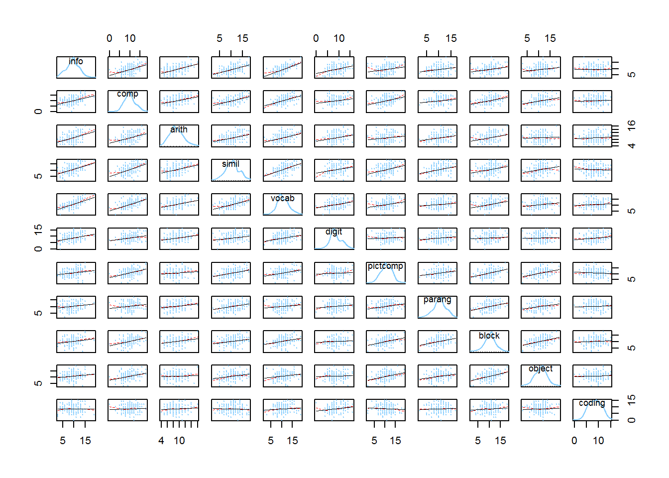

Even with some control over colors and sizes of points/lines, this SPLOM probably has too many variables to be effective - each plot is very small. Nonetheless, the sense of fairly linear relationships among all pairs is somewhat apparent, as is the relative univariate normality of each of the eleven.

Note that the image can be enlarged if the reader is using a pdf version of this document simply by using the increase/decrease size capability of pdf readers. If the user is reading an html version of this document, then try to do a right mouse click on the image and “view image” (in Windows). Then the image can be increased in size in a browser.

2.4 Covariances and Zero Order Correlations

The covariance matrix is the basic input for the CFA algorithms outlined in later chapters.

covmatrix1 <- round(cov(wisc2),digits=3)
knitr::kable(covmatrix1,booktabs=TRUE,format="markdown")

	info	comp	arith	simil	vocab	digit	pictcomp	parang	block	object	coding
info	8.481	4.034	3.322	4.758	5.338	2.720	1.965	1.561	1.808	1.531	0.059
comp	4.034	8.793	2.684	4.816	4.621	1.891	3.540	1.471	2.966	2.718	0.517
arith	3.322	2.684	5.322	2.713	2.621	1.678	1.052	1.391	1.701	0.282	0.598
simil	4.758	4.816	2.713	10.136	5.022	2.234	3.450	2.524	2.255	2.433	-0.372
vocab	5.338	4.621	2.621	5.022	8.601	2.334	2.456	1.031	2.364	1.546	0.842
digit	2.720	1.891	1.678	2.234	2.334	7.313	0.597	1.066	0.533	0.267	1.344
pictcomp	1.965	3.540	1.052	3.450	2.456	0.597	8.610	1.941	3.038	3.032	-0.605
parang	1.561	1.471	1.391	2.524	1.031	1.066	1.941	7.074	2.532	1.916	0.289
block	1.808	2.966	1.701	2.255	2.364	0.533	3.038	2.532	7.343	3.077	0.832
object	1.531	2.718	0.282	2.433	1.546	0.267	3.032	1.916	3.077	8.088	0.433
coding	0.059	0.517	0.598	-0.372	0.842	1.344	-0.605	0.289	0.832	0.433	8.249

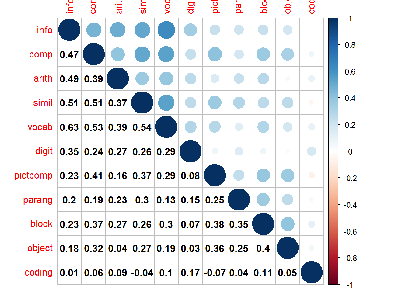
We can use the Corrplot package to produce a useful combination of a schematic and correlation matrix.

mat1 <- cor(wisc2)
corrplot(mat1,type="upper",tl.pos="tp")
corrplot(mat1,add=T,type="lower", method="number",
col="black", diag=FALSE,tl.pos="n", cl.pos="n")

ID	info	comp	arith	simil	vocab	digit	pictcomp	parang	block	object	coding
3	8	7	13	9	12	9	6	11	12	7	9
4	9	6	8	7	11	12	6	8	7	12	14
5	13	18	11	16	15	6	18	8	11	12	9
6	8	11	6	12	9	7	13	4	7	12	11
7	10	3	8	9	12	9	7	7	11	4	10
8	11	7	15	12	10	12	6	12	10	5	10

ID	info	comp	arith	simil	vocab	digit	pictcomp	parang	block	object	coding
3	8	7	13	9	12	9	6	11	12	7	9
4	9	6	8	7	11	12	6	8	7	12	14
5	13	18	11	16	15	6	18	8	11	12	9
6	8	11	6	12	9	7	13	4	7	12	11
7	10	3	8	9	12	9	7	7	11	4	10
8	11	7	15	12	10	12	6	12	10	5	10

ID	info	comp	arith	simil	vocab	digit	pictcomp	parang	block	object	coding
3	8	7	13	9	12	9	6	11	12	7	9
4	9	6	8	7	11	12	6	8	7	12	14
5	13	18	11	16	15	6	18	8	11	12	9
6	8	11	6	12	9	7	13	4	7	12	11
7	10	3	8	9	12	9	7	7	11	4	10
8	11	7	15	12	10	12	6	12	10	5	10