Chapter 3 Using the lavaan package for CFA

One of the primary tools for SEM in R is the lavaan package. It permits path specification with a simple syntax.

3.1 Implement the CFA, First Model

Using the lavaan package, we can implemnt directly the CFA with only a few steps. Since this document contains three different packages’ approach to CFA, the packages used for each will be loaded at that point, so as to not have confusion over common function names.

library(lavaan)

3.1.1 Define and fit the first model

The latent variables and their paths to the manifest variables are initially defined as simple textual specifications. The =~ symbol is the key to defining paths. We have two latent variables and no manifest variable has duplicate paths from both latents. This is a so-called “simple structure.”

Note that this text string uses variable names that match what is in the wisc2 data set.

wisc.model1 <- "verbal  =~ info + comp + arith + simil + vocab + digit 
                 performance =~ pictcomp + parang + block + object + coding"

Fit the model and obtain the basic summary. Note that in this default approach, the latent factors are permitted to covary and the model estimates this covariance.

One R syntax note….. the format here to call the cfa function (lavaan::cfa(.....)) is employed to ensure no ambiguity that the correct cfa function is the one from the lavaan package. This precludes confusion when multiple packages contain functions with the same name as is the case with both lavaan and sem which is also used in this document. Even though sem is loaded later in this document, if there is a chance that it may simultaneously exist in the R environment with lavaan then the approach here is safer.

fit1 <- lavaan::cfa(wisc.model1, data=wisc2,std.lv=TRUE)
summary(fit1, fit.measures=T,standardized=T)

## lavaan 0.6-3 ended normally after 24 iterations
## 
##   Optimization method                           NLMINB
##   Number of free parameters                         23
## 
##   Number of observations                           175
## 
##   Estimator                                         ML
##   Model Fit Test Statistic                      70.640
##   Degrees of freedom                                43
##   P-value (Chi-square)                           0.005
## 
## Model test baseline model:
## 
##   Minimum Function Test Statistic              519.204
##   Degrees of freedom                                55
##   P-value                                        0.000
## 
## User model versus baseline model:
## 
##   Comparative Fit Index (CFI)                    0.940
##   Tucker-Lewis Index (TLI)                       0.924
## 
## Loglikelihood and Information Criteria:
## 
##   Loglikelihood user model (H0)              -4491.822
##   Loglikelihood unrestricted model (H1)      -4456.502
## 
##   Number of free parameters                         23
##   Akaike (AIC)                                9029.643
##   Bayesian (BIC)                              9102.433
##   Sample-size adjusted Bayesian (BIC)         9029.600
## 
## Root Mean Square Error of Approximation:
## 
##   RMSEA                                          0.061
##   90 Percent Confidence Interval          0.033  0.085
##   P-value RMSEA <= 0.05                          0.233
## 
## Standardized Root Mean Square Residual:
## 
##   SRMR                                           0.059
## 
## Parameter Estimates:
## 
##   Information                                 Expected
##   Information saturated (h1) model          Structured
##   Standard Errors                             Standard
## 
## Latent Variables:
##                    Estimate  Std.Err  z-value  P(>|z|)   Std.lv  Std.all
##   verbal =~                                                             
##     info              2.206    0.200   11.029    0.000    2.206    0.760
##     comp              2.042    0.210    9.709    0.000    2.042    0.691
##     arith             1.300    0.172    7.555    0.000    1.300    0.565
##     simil             2.232    0.225    9.940    0.000    2.232    0.703
##     vocab             2.250    0.200   11.225    0.000    2.250    0.770
##     digit             1.053    0.212    4.967    0.000    1.053    0.390
##   performance =~                                                        
##     pictcomp          1.742    0.242    7.187    0.000    1.742    0.595
##     parang            1.253    0.224    5.582    0.000    1.253    0.473
##     block             1.846    0.222    8.311    0.000    1.846    0.683
##     object            1.605    0.236    6.800    0.000    1.605    0.566
##     coding            0.207    0.254    0.814    0.416    0.207    0.072
## 
## Covariances:
##                    Estimate  Std.Err  z-value  P(>|z|)   Std.lv  Std.all
##   verbal ~~                                                             
##     performance       0.589    0.075    7.814    0.000    0.589    0.589
## 
## Variances:
##                    Estimate  Std.Err  z-value  P(>|z|)   Std.lv  Std.all
##    .info              3.566    0.507    7.034    0.000    3.566    0.423
##    .comp              4.572    0.585    7.815    0.000    4.572    0.523
##    .arith             3.602    0.420    8.571    0.000    3.602    0.681
##    .simil             5.096    0.662    7.702    0.000    5.096    0.506
##    .vocab             3.487    0.506    6.886    0.000    3.487    0.408
##    .digit             6.162    0.680    9.056    0.000    6.162    0.848
##    .pictcomp          5.526    0.757    7.296    0.000    5.526    0.646
##    .parang            5.463    0.658    8.298    0.000    5.463    0.777
##    .block             3.894    0.640    6.083    0.000    3.894    0.533
##    .object            5.467    0.719    7.600    0.000    5.467    0.680
##    .coding            8.159    0.874    9.335    0.000    8.159    0.995
##     verbal            1.000                               1.000    1.000
##     performance       1.000                               1.000    1.000

3.1.2 Obtain coefficients

It is possible to obtain the output from the above summary function that does not contain the parameter coefficients part of the table. If that had been the implementation, then the coefficients can be obtained simply, but it is better to obtain the full table of parameter estimates and errors, etc.

# obtain only the coefficients
kable(coef(fit1), booktabs=TRUE, format="markdown")

3.1.3 Complete parameter listing

Instead of directly printing the parameter table, I prefer to reformat it with kable when using R Markdown. Without using kable, the code would be the following:

parameterEstimates(fit1,standardized=T)

Format the table and clean it up using kable.

parameterEstimates(fit1, standardized=TRUE) %>% 
  filter(op == "=~") %>% 
  select('Latent Factor'=lhs, Indicator=rhs, B=est, SE=se, Z=z, 'p-value'=pvalue, Beta=std.all) %>% 
  knitr::kable(digits = 3, booktabs=TRUE, format="markdown", caption="Factor Loadings")

Latent Factor	Indicator	B	SE	Z	p-value	Beta
verbal	info	2.206	0.200	11.029	0.000	0.760
verbal	comp	2.042	0.210	9.709	0.000	0.691
verbal	arith	1.300	0.172	7.555	0.000	0.565
verbal	simil	2.232	0.225	9.940	0.000	0.703
verbal	vocab	2.250	0.200	11.225	0.000	0.770
verbal	digit	1.053	0.212	4.967	0.000	0.390
performance	pictcomp	1.742	0.242	7.187	0.000	0.595
performance	parang	1.253	0.224	5.582	0.000	0.473
performance	block	1.846	0.222	8.311	0.000	0.683
performance	object	1.605	0.236	6.800	0.000	0.566
performance	coding	0.207	0.254	0.814	0.416	0.072

3.1.4 Residuals correlation matrix

Residuals can be examined.

cor_table <- residuals(fit1, type = "cor")$cov
#cor_table[upper.tri(cor_table)] <-  # erase the upper triangle
#diag(cor_table) <- NA # erase the diagonal 0's
knitr::kable(cor_table, digits=3,format="markdown", booktabs=TRUE) # makes a nice table and rounds everyhing to 2 digits

	info	comp	arith	simil	vocab	digit	pictcomp	parang	block	object	coding
info	0.000	-0.058	0.065	-0.021	0.040	0.049	-0.036	-0.010	-0.076	-0.068	-0.025
comp	-0.058	0.000	0.002	0.025	0.000	-0.034	0.165	-0.006	0.091	0.092	0.031
arith	0.065	0.002	0.000	-0.028	-0.047	0.048	-0.043	0.069	0.045	-0.145	0.066
simil	-0.021	0.025	-0.028	0.000	-0.003	-0.015	0.123	0.102	-0.021	0.034	-0.071
vocab	0.040	0.000	-0.047	-0.003	0.000	-0.006	0.016	-0.082	-0.012	-0.071	0.067
digit	0.049	-0.034	0.048	-0.015	-0.006	0.000	-0.062	0.040	-0.084	-0.095	0.156
pictcomp	-0.036	0.165	-0.043	0.123	0.016	-0.062	0.000	-0.033	-0.025	0.026	-0.115
parang	-0.010	-0.006	0.069	0.102	-0.082	0.040	-0.033	0.000	0.028	-0.014	0.004
block	-0.076	0.091	0.045	-0.021	-0.012	-0.084	-0.025	0.028	0.000	0.013	0.058
object	-0.068	0.092	-0.145	0.034	-0.071	-0.095	0.026	-0.014	0.013	0.000	0.012
coding	-0.025	0.031	0.066	-0.071	0.067	0.156	-0.115	0.004	0.058	0.012	0.000

3.1.5 Plot the residuals.

norm plot

# extract the residuals from the fit1 model
# get rid of the duplicates and diagonal values
# create a vector for a
res1 <- residuals(fit1, type = "cor")$cov
res1[upper.tri(res1,diag=T)] <- NA
v1 <- as.vector(res1)
v2  <- v1[!is.na(v1)]
qqPlot(v2,id=F)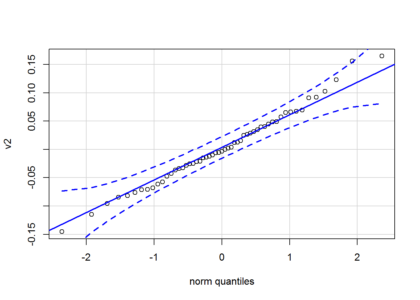

3.1.6 Modification Indices

Modification indices provide……

kable(modificationIndices(fit1, sort.=TRUE, minimum.value=3), booktabs=TRUE, format="markdown")

	lhs	op	rhs	mi	epc	sepc.lv	sepc.all	sepc.nox
32	performance	=~	comp	9.823223	0.9372111	0.9372111	0.3169647	0.3169647
62	arith	~~	object	6.362360	-0.9445341	-0.9445341	-0.2128471	-0.2128471
37	info	~~	comp	5.221423	-0.9847261	-0.9847261	-0.2438796	-0.2438796
81	digit	~~	coding	4.926741	1.2072274	1.2072274	0.1702526	0.1702526
51	comp	~~	pictcomp	4.685434	0.9693124	0.9693124	0.1928391	0.1928391
85	pictcomp	~~	coding	4.574821	-1.2249127	-1.2249127	-0.1824249	-0.1824249
31	performance	=~	info	4.476617	-0.5955241	-0.5955241	-0.2050748	-0.2050748
40	info	~~	vocab	4.402900	0.9124221	0.9124221	0.2587532	0.2587532
73	vocab	~~	parang	4.145852	-0.7977279	-0.7977279	-0.1827712	-0.1827712
38	info	~~	arith	4.133326	0.6970216	0.6970216	0.1944960	0.1944960
67	simil	~~	parang	3.373228	0.8304961	0.8304961	0.1574097	0.1574097
70	simil	~~	coding	3.271062	-0.9560218	-0.9560218	-0.1482698	-0.1482698
66	simil	~~	pictcomp	3.269521	0.8602498	0.8602498	0.1621163	0.1621163

3.1.7 Path Diagram for the bifactor Model 1

The semPlot package provides a capability of drawing path diagrams for cfa and other sem models. The semPaths function will take a cfa model object and draw the diagram, with several options available. The diagram produced here takes control over font/label sizes, display of residuals, and color of paths/coefficients. These and many more control options are available. There is a challenge in producing these path diagrams to have font sizes large enough for most humans to read. I’ve taken control of the font sizes for the “edges” with a cex argument. But this causes overlap in the values if the default layout is used. I found that “circle2” worked best here.

# Note that the base plot, including standardized path coefficients plots positive coefficients green
# and negative coefficients red.  Red-green colorblindness issues anyone?
# I redrew it here to choose a blue and red.  But all the coefficients in this example are
# positive,so they are shown with the skyblue.
# more challenging to use colors other than red and green.  not in this doc
semPaths(fit1, residuals=F,sizeMan=7,"std",
         posCol=c("skyblue4", "red"),
         #edge.color="skyblue4",
         edge.label.cex=1.2,layout="circle2")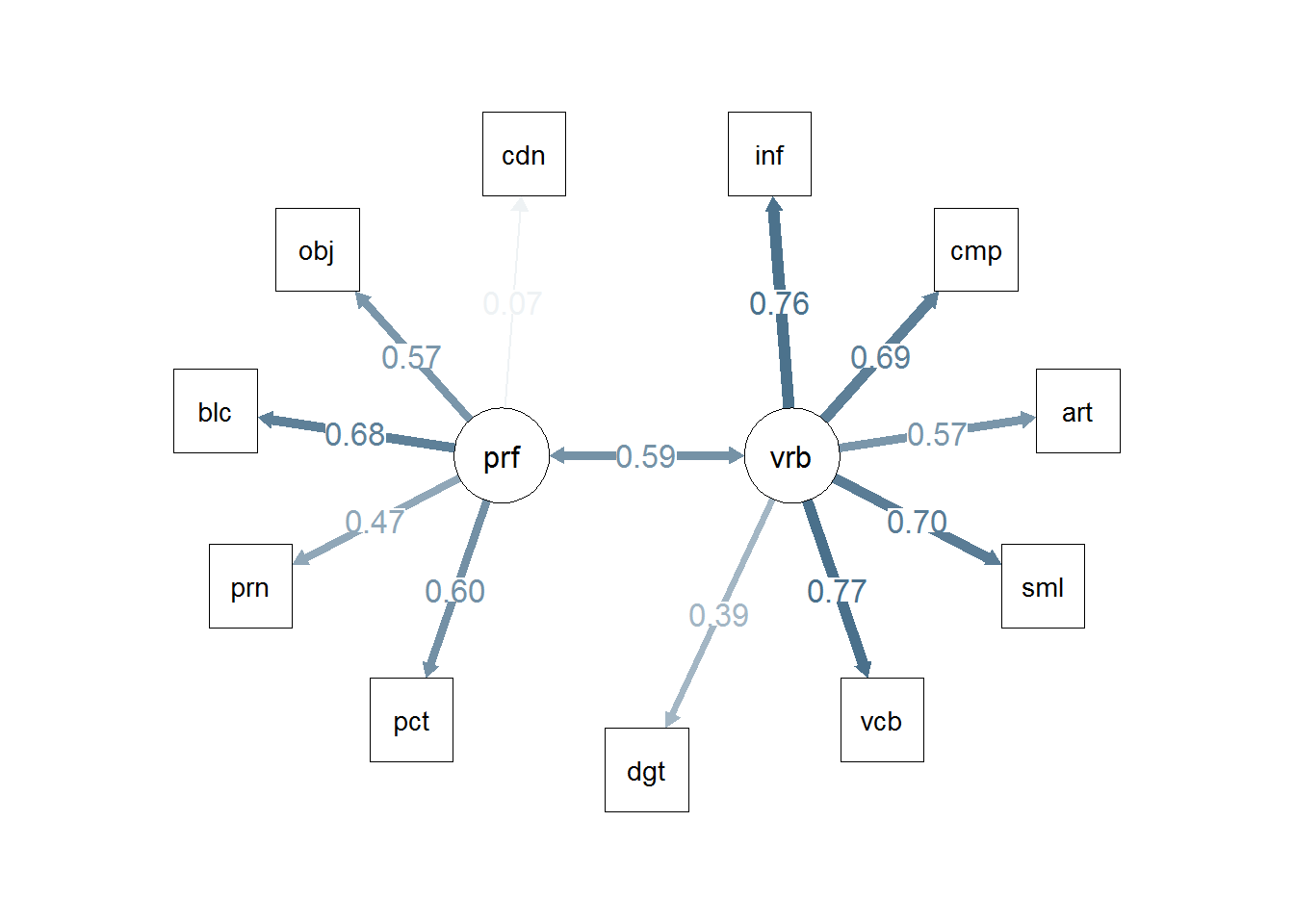

# or we could draw the paths in such  a way to include the residuals:
#semPaths(fit1, sizeMan=7,"std",edge.color="skyblue4",edge.label.cex=1,layout="circle2")
# the base path diagram can be drawn much more simply:
#semPaths(fit1)
# or
semPaths(fit1,"std")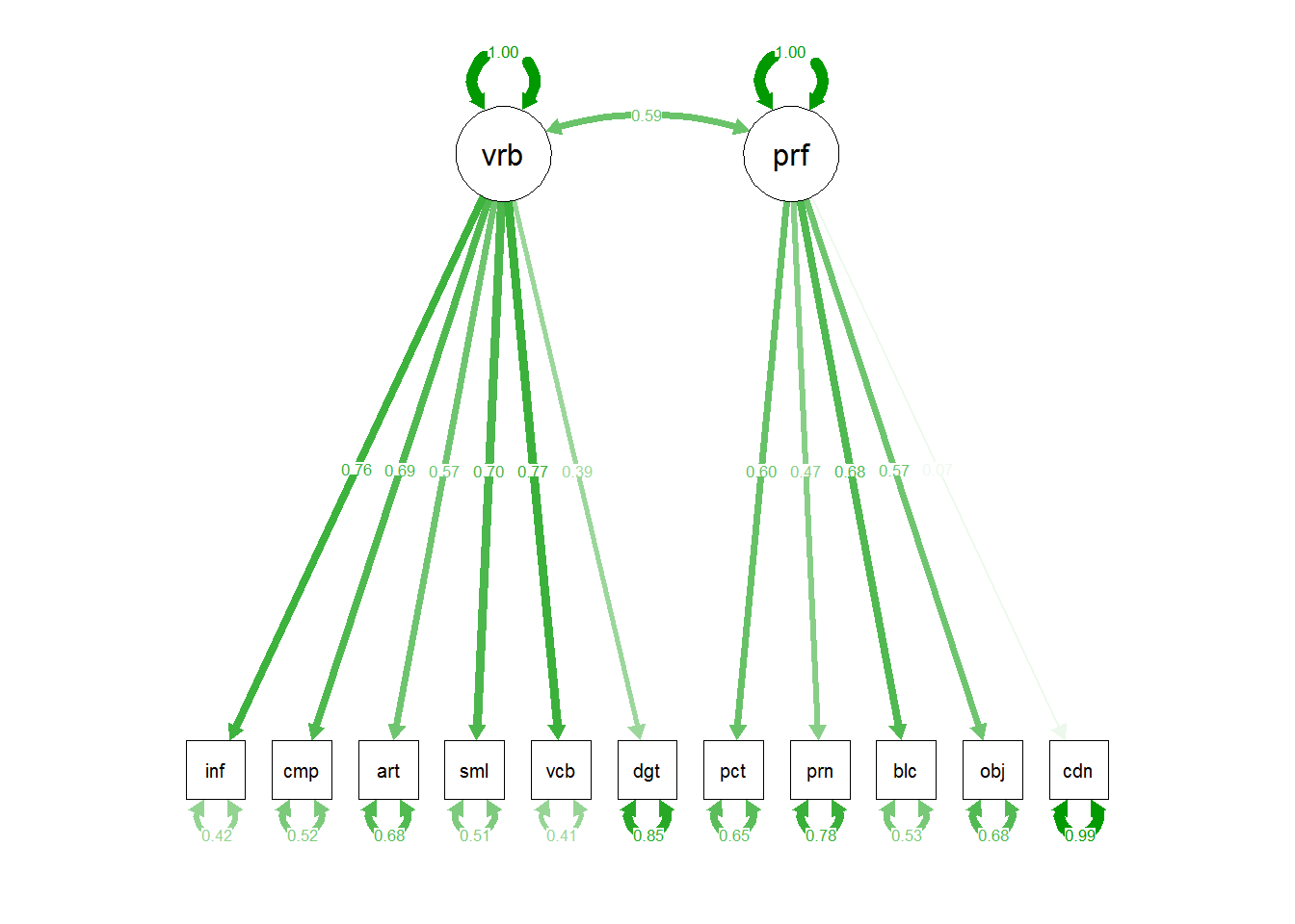

3.1.8 orthognal fit comparison

Compare to a one factor solution.

fit1orth <- lavaan::cfa(wisc.model1, data=wisc1,orthogonal=T)
kable(anova(fit1,fit1orth), booktabs=TRUE, format="markdown")

	Df	AIC	BIC	Chisq	Chisq diff	Df diff	Pr(>Chisq)
fit1	43	9029.643	9102.433	70.63957	NA	NA	NA
fit1orth	44	9065.614	9135.239	108.60977	37.97019	1	0

3.2 Generate a second model and compare

Next, generate a second CFA model. Thre are theoretical reasons why paths from both latent factors to “comp” might be warranted. The “comp” variable also has the largest Modification index in the first model. This second modelimplements this one-path/parmaeter change.

3.2.1 Add a path (Perf to comp) and Fit the second CFA model

Define the addditional path in the model text string.

wisc.model2 <- 'verbal  =~ info + comp + arith + simil + vocab + digit 
                performance =~ pictcomp + parang + block + object + coding + comp'

Fit the model and obtain the basic summary

fit2 <- lavaan::cfa(wisc.model2, data=wisc1,std.lv=TRUE)
summary(fit2, fit.measures=T,standardized=T)

## lavaan 0.6-3 ended normally after 26 iterations
## 
##   Optimization method                           NLMINB
##   Number of free parameters                         24
## 
##   Number of observations                           175
## 
##   Estimator                                         ML
##   Model Fit Test Statistic                      60.642
##   Degrees of freedom                                42
##   P-value (Chi-square)                           0.031
## 
## Model test baseline model:
## 
##   Minimum Function Test Statistic              519.204
##   Degrees of freedom                                55
##   P-value                                        0.000
## 
## User model versus baseline model:
## 
##   Comparative Fit Index (CFI)                    0.960
##   Tucker-Lewis Index (TLI)                       0.947
## 
## Loglikelihood and Information Criteria:
## 
##   Loglikelihood user model (H0)              -4486.823
##   Loglikelihood unrestricted model (H1)      -4456.502
## 
##   Number of free parameters                         24
##   Akaike (AIC)                                9021.645
##   Bayesian (BIC)                              9097.600
##   Sample-size adjusted Bayesian (BIC)         9021.600
## 
## Root Mean Square Error of Approximation:
## 
##   RMSEA                                          0.050
##   90 Percent Confidence Interval          0.016  0.077
##   P-value RMSEA <= 0.05                          0.465
## 
## Standardized Root Mean Square Residual:
## 
##   SRMR                                           0.054
## 
## Parameter Estimates:
## 
##   Information                                 Expected
##   Information saturated (h1) model          Structured
##   Standard Errors                             Standard
## 
## Latent Variables:
##                    Estimate  Std.Err  z-value  P(>|z|)   Std.lv  Std.all
##   verbal =~                                                             
##     info              2.256    0.199   11.318    0.000    2.256    0.777
##     comp              1.491    0.254    5.877    0.000    1.491    0.504
##     arith             1.307    0.172    7.584    0.000    1.307    0.568
##     simil             2.205    0.226    9.748    0.000    2.205    0.695
##     vocab             2.273    0.201   11.329    0.000    2.273    0.777
##     digit             1.075    0.212    5.068    0.000    1.075    0.399
##   performance =~                                                        
##     pictcomp          1.790    0.239    7.495    0.000    1.790    0.612
##     parang            1.189    0.224    5.317    0.000    1.189    0.448
##     block             1.823    0.219    8.334    0.000    1.823    0.675
##     object            1.633    0.233    7.010    0.000    1.633    0.576
##     coding            0.200    0.253    0.793    0.428    0.200    0.070
##     comp              0.884    0.266    3.324    0.001    0.884    0.299
## 
## Covariances:
##                    Estimate  Std.Err  z-value  P(>|z|)   Std.lv  Std.all
##   verbal ~~                                                             
##     performance       0.533    0.081    6.594    0.000    0.533    0.533
## 
## Variances:
##                    Estimate  Std.Err  z-value  P(>|z|)   Std.lv  Std.all
##    .info              3.343    0.502    6.665    0.000    3.343    0.396
##    .comp              4.331    0.554    7.819    0.000    4.331    0.495
##    .arith             3.584    0.420    8.533    0.000    3.584    0.677
##    .simil             5.217    0.675    7.726    0.000    5.217    0.518
##    .vocab             3.383    0.508    6.655    0.000    3.383    0.396
##    .digit             6.116    0.677    9.032    0.000    6.116    0.841
##    .pictcomp          5.358    0.741    7.231    0.000    5.358    0.626
##    .parang            5.620    0.663    8.480    0.000    5.620    0.799
##    .block             3.979    0.623    6.385    0.000    3.979    0.545
##    .object            5.376    0.707    7.603    0.000    5.376    0.668
##    .coding            8.162    0.874    9.337    0.000    8.162    0.995
##     verbal            1.000                               1.000    1.000
##     performance       1.000                               1.000    1.000

3.2.2 Obtain coefficients

Coefficients can be obtained simply with the coef function, but it is better to do the full parameter listing in the next section

knitr::kable(coef(fit2),booktabs=TRUE, format="markdown")

It is simple to obtain the full parameter list, but I prefer to use kable for tables when I can.

parameterEstimates(fit2,standardized=TRUE)

Reformat the table and clean it up by using kable.

parameterEstimates(fit2, standardized=TRUE) %>% 
  filter(op == "=~") %>% 
  select('Latent Factor'=lhs, Indicator=rhs, B=est, SE=se, Z=z, 'p-value'=pvalue, Beta=std.all) %>% 
  knitr::kable(digits = 3, format="markdown", booktabs=TRUE, caption="Factor Loadings")

Latent Factor	Indicator	B	SE	Z	p-value	Beta
verbal	info	2.256	0.199	11.318	0.000	0.777
verbal	comp	1.491	0.254	5.877	0.000	0.504
verbal	arith	1.307	0.172	7.584	0.000	0.568
verbal	simil	2.205	0.226	9.748	0.000	0.695
verbal	vocab	2.273	0.201	11.329	0.000	0.777
verbal	digit	1.075	0.212	5.068	0.000	0.399
performance	pictcomp	1.790	0.239	7.495	0.000	0.612
performance	parang	1.189	0.224	5.317	0.000	0.448
performance	block	1.823	0.219	8.334	0.000	0.675
performance	object	1.633	0.233	7.010	0.000	0.576
performance	coding	0.200	0.253	0.793	0.428	0.070
performance	comp	0.884	0.266	3.324	0.001	0.299

3.2.3 Residuals correlation matrix

Residuals can be examined.

cor_table2 <- residuals(fit2, type = "cor")$cov

#cor_table[upper.tri(cor_table)] <-  # erase the upper triangle
#diag(cor_table) <- NA # erase the diagonal 0's
knitr::kable(cor_table2, digits=3,format="markdown",booktabs=TRUE) # makes a nice table and rounds everyhing to 2 digits

	info	comp	arith	simil	vocab	digit	pictcomp	parang	block	object	coding
info	0.000	-0.049	0.053	-0.026	0.021	0.036	-0.023	0.016	-0.050	-0.054	-0.022
comp	-0.049	0.000	0.015	0.049	0.015	-0.029	0.059	-0.068	-0.014	-0.005	0.021
arith	0.053	0.015	0.000	-0.025	-0.054	0.043	-0.030	0.091	0.068	-0.131	0.069
simil	-0.026	0.049	-0.025	0.000	-0.002	-0.017	0.143	0.132	0.012	0.056	-0.067
vocab	0.021	0.015	-0.054	-0.002	0.000	-0.016	0.032	-0.054	0.018	-0.053	0.071
digit	0.036	-0.029	0.043	-0.017	-0.016	0.000	-0.055	0.053	-0.071	-0.088	0.158
pictcomp	-0.023	0.059	-0.030	0.143	0.032	-0.055	0.000	-0.025	-0.031	0.011	-0.115
parang	0.016	-0.068	0.091	0.132	-0.054	0.053	-0.025	0.000	0.049	-0.005	0.006
block	-0.050	-0.014	0.068	0.012	0.018	-0.071	-0.031	0.049	0.000	0.011	0.060
object	-0.054	-0.005	-0.131	0.056	-0.053	-0.088	0.011	-0.005	0.011	0.000	0.013
coding	-0.022	0.021	0.069	-0.067	0.071	0.158	-0.115	0.006	0.060	0.013	0.000

3.2.4 Modification Indices for Model 2

Modification indices provide………………..

kable(modificationIndices(fit2, sort.=TRUE, minimum.value=3), booktabs=TRUE, format="markdown")

	lhs	op	rhs	mi	epc	sepc.lv	sepc.all	sepc.nox
34	performance	=~	simil	6.763658	0.7945731	0.7945731	0.2502971	0.2502971
62	arith	~~	object	5.551414	-0.8741210	-0.8741210	-0.1991496	-0.1991496
81	digit	~~	coding	4.975650	1.2098255	1.2098255	0.1712424	0.1712424
85	pictcomp	~~	coding	4.742106	-1.2338394	-1.2338394	-0.1865857	-0.1865857
66	simil	~~	pictcomp	3.810872	0.9252477	0.9252477	0.1750135	0.1750135
52	comp	~~	parang	3.768775	-0.8524973	-0.8524973	-0.1727905	-0.1727905
73	vocab	~~	parang	3.689972	-0.7528236	-0.7528236	-0.1726510	-0.1726510
67	simil	~~	parang	3.578938	0.8683482	0.8683482	0.1603695	0.1603695
57	arith	~~	vocab	3.377455	-0.6406313	-0.6406313	-0.1839884	-0.1839884
61	arith	~~	block	3.256929	0.6099258	0.6099258	0.1615230	0.1615230
38	info	~~	arith	3.216572	0.6208828	0.6208828	0.1793789	0.1793789
70	simil	~~	coding	3.165192	-0.9489408	-0.9489408	-0.1454290	-0.1454290

3.2.5 Path Diagram for Model 2

The semPlot package provides a capability of drawing path diagrams for cfa and other sem models. The semPaths function will take a cfa model object and draw the diagram, with several options available. The diagram produced here takes control over font/label sizes, display of residuals, and color of paths/coefficients. These and many more control options are available. There is a challenge in producing these path diagrams to have font sizes large enough for most humans to read. I’ve taken control of the font sizes for the “edges” with a cex argument. But this causes overlap in the values if the default layout is used. I found that “circle2” worked best here.

# Note that the base plot, including standardized path coefficients plots positive coefficients green
# and negative coefficients red.  Red-green colorblindness issues anyone?
# I redrew it here to choose a blue and red.  But all the coefficients in this example are
# positive,so they are shown with the skyblue.
# more challenging to use colors other than red and green.  not in this doc
semPaths(fit2, residuals=F,sizeMan=7,"std",
         posCol=c("skyblue4", "red"),
         #edge.color="skyblue4",
         edge.label.cex=1.2,layout="circle2")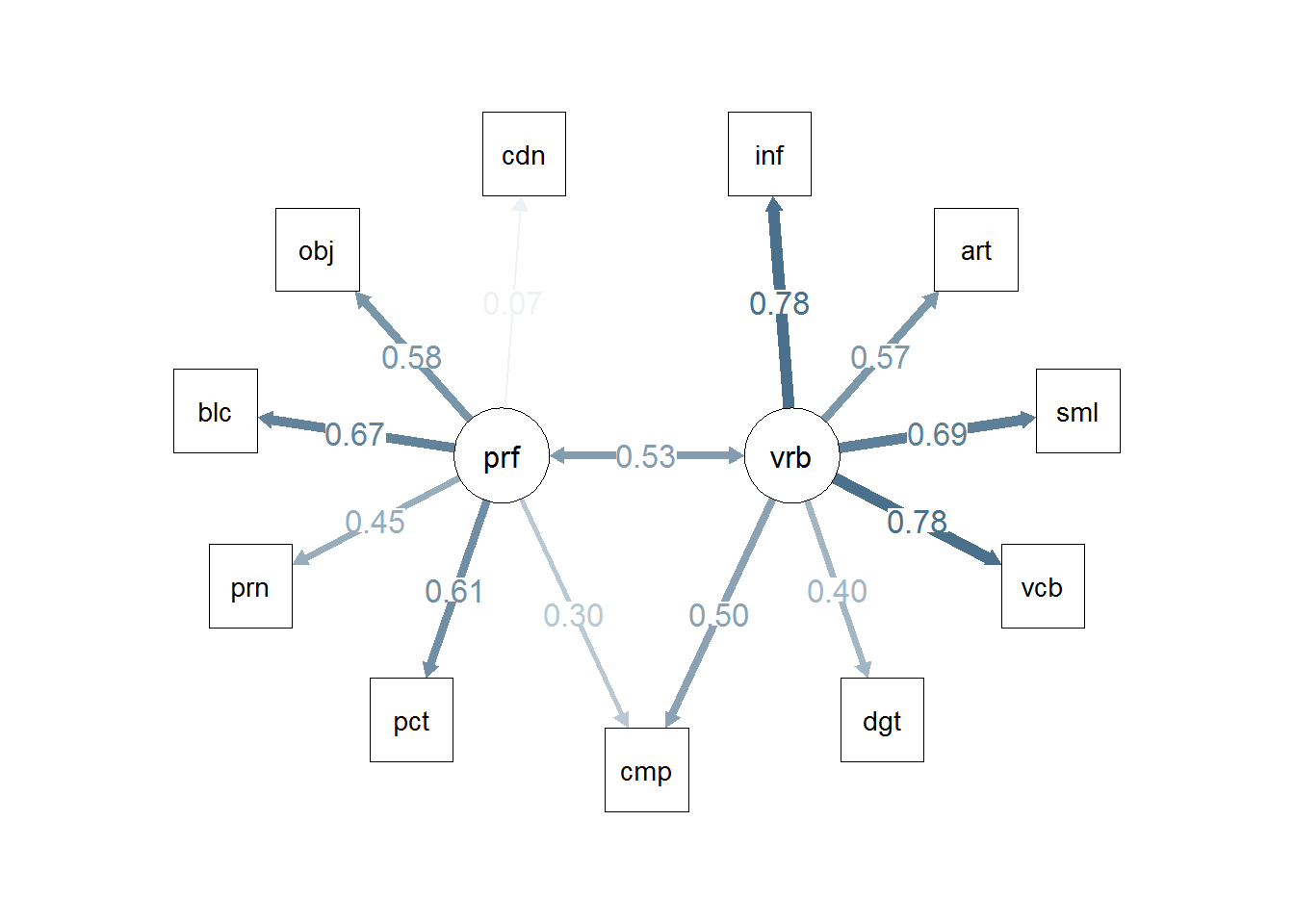

# or we could draw the paths in such  a way to include the residuals:
#semPaths(fit1, sizeMan=7,"std",edge.color="skyblue4",edge.label.cex=1,layout="circle2")
# the base path diagram can be drawn much more simply:
#semPaths(fit2)
# or
semPaths(fit2,"std")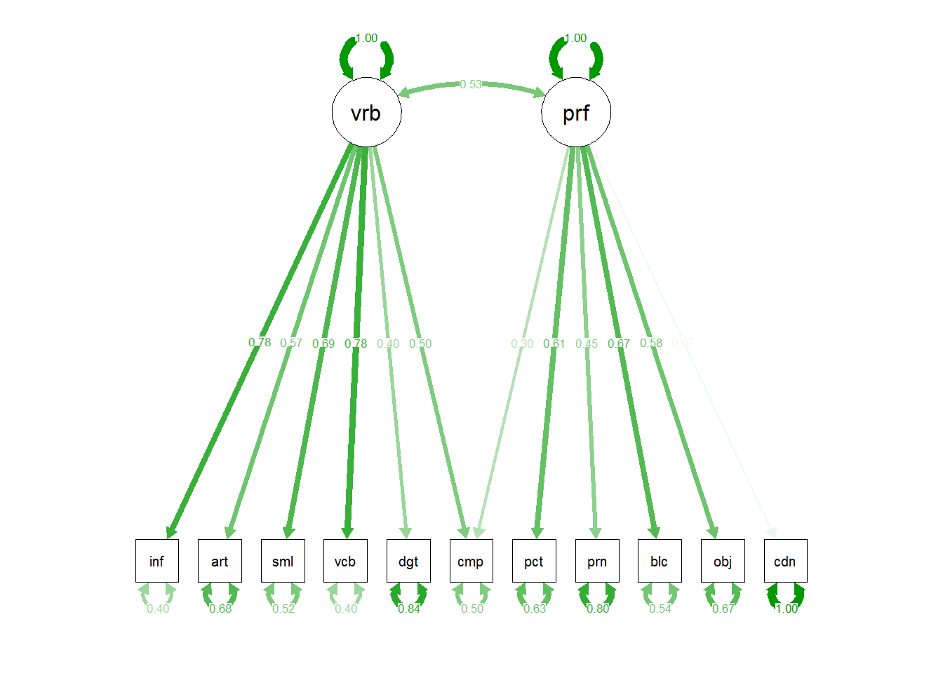

3.3 Compare Model 1 and Model 2

Model 1 is first/base. Model 2 adds a path from Perf to comp… Compare these models.

kable(anova(fit1,fit2), booktabs=TRUE, format="markdown")

	Df	AIC	BIC	Chisq	Chisq diff	Df diff	Pr(>Chisq)
fit2	42	9021.645	9097.600	60.64158	NA	NA	NA
fit1	43	9029.643	9102.433	70.63957	9.997993	1	0.0015671

3.4 An additional perspective on estimation and optimization

Subtle differences in algorithmic strategies for Structural Equation Modeling exist among software packages. Users are often familiar with only the default approaches and will only be moved to learn other approaches when the default approach fails to converge or produces problematic models. The student first confronted with these methods will often assume that the same SEM model evauated in different software (e.g., LISREL, MPlus, EQS, lavaan, sem, OpenMx) will produce the same model outcome. This may not be a safe assumption. Different “dialects” exist for the various software products. The commercial products may use algorithms that are proprietary and not available to understand their approach. The open source products (e.g., lavaan) have made source code available for inspection.

The perceptive reader will notice that the default solutions given by the three R packages employed in this document (lavaan, sem, OpenMx) all give the same values for parameter estimates and goodnes of fit statistics for the same two models run with each. However, there are slight differences in these quantities compared to the published LISREL analysis of the same data in the Tabachnik, et al textbook ((2019)). Other readers will have noticed that the LISREL output in this textbook matches SAS output that they may have seen with class coverage of the CFA topic. The R packages, while agreeing with each other, vary slightly from the LISREL and SAS values. The degree of difference is slight, but its existence may puzzle some students. The answer to understanding these differences goes well beyond the scope of this document and involves an advanced understanding of the computational algorithms employed. Even though all of the approaches are Maximum Liklihood methods some optimization and estimation strategies can differ.

The lavaan package permits some insight into this with one of the argments available for the cfa function used in this chapter. The reader might want to examine the help docs for this function: ?cfa. That help page directs readers to another help document on Lavaan Options (lavoptions). There, one can find an argument that can be passed to cfa, called “mimic”. Here is the text from that section, describing the various “mimic” possibilities:

“If”Mplus“, an attempt is made to mimic the Mplus program. If”EQS“, an attempt is made to mimic the EQS program. If”default“, the value is (currently) set to to”lavaan“, which is very close to”Mplus“.”

The reader may have been exposed to a SAS Proc Calis approach to this problem that employed the default Method called LINEQS. The following rerun of the first model from this chapter above, employs the mimic argument to be specified as “EQS”. The product of this model is a set of parameter values and fit statistics (e.g., Chi Sq) that match the SAS output (and the Tabachnick et al LISREL output) exactly. Demonstrating the equivalence with the addition of the mimic argument does not fully explain why such differences originally existed, but that, again, is well beyond the scope of this document. The reference section to this document includes some articles that address these differences (El-Sheikh et al., 2017; Narayanan, 2012). Rosseel (2012) has discussed use of the ‘mimic’ function that guides lavaan to emulate the approach of some of the commercial products. His website is also a valuable resource on this [http://lavaan.ugent.be/].

wisc.model1 <- "verbal  =~ info + comp + arith + simil + vocab + digit 
                 performance =~ pictcomp + parang + block + object + coding"

fit1eqs <- lavaan::cfa(wisc.model1, data=wisc2,std.lv=TRUE, mimic="EQS")
summary(fit1eqs, fit.measures=T,standardized=T)

## lavaan 0.6-3 ended normally after 25 iterations
## 
##   Optimization method                           NLMINB
##   Number of free parameters                         23
## 
##   Number of observations                           175
## 
##   Estimator                                         ML
##   Model Fit Test Statistic                      70.236
##   Degrees of freedom                                43
##   P-value (Chi-square)                           0.005
## 
## Model test baseline model:
## 
##   Minimum Function Test Statistic              516.237
##   Degrees of freedom                                55
##   P-value                                        0.000
## 
## User model versus baseline model:
## 
##   Comparative Fit Index (CFI)                    0.941
##   Tucker-Lewis Index (TLI)                       0.924
## 
## Loglikelihood and Information Criteria:
## 
##   Loglikelihood user model (H0)              -4497.337
##   Loglikelihood unrestricted model (H1)      -4462.018
## 
##   Number of free parameters                         23
##   Akaike (AIC)                                9040.675
##   Bayesian (BIC)                              9113.465
##   Sample-size adjusted Bayesian (BIC)         9040.631
## 
## Root Mean Square Error of Approximation:
## 
##   RMSEA                                          0.060
##   90 Percent Confidence Interval          0.033  0.085
##   P-value RMSEA <= 0.05                          0.239
## 
## Standardized Root Mean Square Residual:
## 
##   SRMR                                           0.059
## 
## Parameter Estimates:
## 
##   Information                                 Expected
##   Information saturated (h1) model          Structured
##   Standard Errors                             Standard
## 
## Latent Variables:
##                    Estimate  Std.Err  z-value  P(>|z|)   Std.lv  Std.all
##   verbal =~                                                             
##     info              2.212    0.201   10.997    0.000    2.212    0.760
##     comp              2.048    0.212    9.682    0.000    2.048    0.691
##     arith             1.304    0.173    7.534    0.000    1.304    0.565
##     simil             2.238    0.226    9.911    0.000    2.238    0.703
##     vocab             2.257    0.202   11.193    0.000    2.257    0.770
##     digit             1.056    0.213    4.952    0.000    1.056    0.390
##   performance =~                                                        
##     pictcomp          1.747    0.244    7.166    0.000    1.747    0.595
##     parang            1.257    0.226    5.566    0.000    1.257    0.473
##     block             1.851    0.223    8.287    0.000    1.851    0.683
##     object            1.609    0.237    6.780    0.000    1.609    0.566
##     coding            0.208    0.256    0.811    0.417    0.208    0.072
## 
## Covariances:
##                    Estimate  Std.Err  z-value  P(>|z|)   Std.lv  Std.all
##   verbal ~~                                                             
##     performance       0.589    0.076    7.792    0.000    0.589    0.589
## 
## Variances:
##                    Estimate  Std.Err  z-value  P(>|z|)   Std.lv  Std.all
##    .info              3.586    0.511    7.014    0.000    3.586    0.423
##    .comp              4.599    0.590    7.793    0.000    4.599    0.523
##    .arith             3.623    0.424    8.547    0.000    3.623    0.681
##    .simil             5.125    0.667    7.680    0.000    5.125    0.506
##    .vocab             3.507    0.511    6.866    0.000    3.507    0.408
##    .digit             6.198    0.686    9.030    0.000    6.198    0.848
##    .pictcomp          5.558    0.764    7.276    0.000    5.558    0.646
##    .parang            5.494    0.664    8.275    0.000    5.494    0.777
##    .block             3.916    0.646    6.066    0.000    3.916    0.533
##    .object            5.499    0.726    7.578    0.000    5.499    0.680
##    .coding            8.206    0.882    9.309    0.000    8.206    0.995
##     verbal            1.000                               1.000    1.000
##     performance       1.000                               1.000    1.000