Chapter 4 Using the sem package for CFA
In this chapter, we use the sem package to implement the same two CFA analyses that we produced with lavaan in chapter 3. sem provides an equally simple way to obtain the models and only the basics are shown here. The code in this chapter is modeled after a document by James Steiger
4.1 Example one
Once again, the bifactor model with Verbal and Performance factors is specified. Each manifest factor has a path from only one of the two factors.
4.1.1 Data Setup
In sem, it is helpful to have covariance and correlation matrices available as objects, as well ans a sample size object.
# same data file and extraction of the wisc2 data frame with only the 11 manifests
#wisc1 <- read.csv("wisc1.csv")
#wisc2 <- wisc1[,2:12]
# covariance and correlation matrices are saved as objects
covwisc <- cov(wisc2)
corwisc <-cor(wisc2)
# list of manifest variables for potential use
manifests <- names(wisc2)
# this gives an object that is the sample size
wobs <- length(wisc2)
We also need to load the package.
4.1.2 Define the first model
In sem, the structure of the model is created with a text string to define the paths. The specifyModel function permits this in several ways. The simplest is to enter text as an argument. Some explanation of the strucure is needed.
- Each line defines a path, a label for the parameter, and the starting value for the parameter value.
- This is symbolized as:
, , . - Note that paths can be double or single-headed arrows.
- The unique name specified by the parameter symbol is for free parameters.
- If the parameter value is NA, then its starting point value is system determined.
- A numerical value following the NA can fix a variance at the value. E.g.,: F1 <-> F1, NA, 1 would fix the factor variance a 1.
- Unique variances can be specified for manifest variables. e.g.,: manifest1 <-> manifest1, e1, NA. If they are not specified, they default to “free to vary”
- Factors can be set to a fixed relationship to each other, e.g, 0, or 1. Or they can be left free (estimable) as in the example here.
# this text could have been saved in a file and read in with the file argument to be efficient
# commented here to show the argument options
# m1.model <- specifyModel(file="sem1.txt")
m1.model <- specifyModel(text="
  ## Factor 1 is Verbal
  Verbal -> info, t01, NA
  Verbal -> comp, t02, NA
  Verbal -> arith, t03, NA
  Verbal -> simil, t04, NA
  Verbal -> vocab, t05, NA
  Verbal -> digit, t06, NA
  ## Factor 2 is performance
  Performance -> pictcomp, t07, NA
  Performance -> parang, t08, NA
  Performance -> block, t09, NA
  Performance -> object, t10, NA
  Performance -> coding, t11, NA
  ## Set factor variances
  Verbal <-> Verbal, NA, 1
  Performance <-> Performance, NA, 1
  ## Set factor covariance to be estimable
  Verbal <-> Performance, p1, NA"
)
## NOTE: it is generally simpler to use specifyEquations() or cfa()
## see ?specifyEquations## NOTE: adding 11 variances to the modelThis m1.model is now available to be used in the model function. The first “note” refers to the fact that the model can be specified interactivly (I think). I found it easier to do this way, and more reproducible.
4.1.3 Fit model 1 and examine the results
In this chapter, we will just look at the basics of the model fit and draw the path diagram. Other aspects of the model can be extracted, but are passed over here to save space. The interested reader might try str(m1) to see what is available from the model object.
# all that is required is the model specification, the covariance matrix, and the sample size
m1 <- sem(m1.model,covwisc,175)
options(digits=5)
summary(m1)
##
## Model Chisquare = 70.236 Df = 43 Pr(>Chisq) = 0.0054454
## AIC = 116.24
## BIC = -151.85
##
## Normalized Residuals
## Min. 1st Qu. Median Mean 3rd Qu. Max.
## -1.88413 -0.41375 -0.00001 0.03511 0.45976 2.11208
##
## R-square for Endogenous Variables
## info comp arith simil vocab digit pictcomp parang
## 0.5772 0.4770 0.3193 0.4944 0.5922 0.1524 0.3545 0.2233
## block object coding
## 0.4667 0.3202 0.0052
##
## Parameter Estimates
## Estimate Std Error z value Pr(>|z|)
## t01 2.21249 0.201190 10.99700 3.9507e-28 info <--- Verbal
## t02 2.04806 0.211541 9.68163 3.6090e-22 comp <--- Verbal
## t03 1.30357 0.173035 7.53358 4.9367e-14 arith <--- Verbal
## t04 2.23845 0.225846 9.91142 3.7135e-23 simil <--- Verbal
## t05 2.25691 0.201642 11.19269 4.4281e-29 vocab <--- Verbal
## t06 1.05579 0.213185 4.95244 7.3287e-07 digit <--- Verbal
## t07 1.74699 0.243776 7.16638 7.7008e-13 pictcomp <--- Performance
## t08 1.25683 0.225785 5.56647 2.5995e-08 parang <--- Performance
## t09 1.85123 0.223392 8.28693 1.1621e-16 block <--- Performance
## t10 1.60918 0.237324 6.78052 1.1974e-11 object <--- Performance
## t11 0.20761 0.255890 0.81132 4.1718e-01 coding <--- Performance
## p1 0.58883 0.075569 7.79198 6.5965e-15 Performance <--> Verbal
## V[info] 3.58620 0.511281 7.01414 2.3137e-12 info <--> info
## V[comp] 4.59856 0.590106 7.79277 6.5556e-15 comp <--> comp
## V[arith] 3.62254 0.423850 8.54675 1.2660e-17 arith <--> arith
## V[simil] 5.12484 0.667296 7.68001 1.5908e-14 simil <--> simil
## V[vocab] 3.50720 0.510787 6.86626 6.5906e-12 vocab <--> vocab
## V[digit] 6.19783 0.686345 9.03020 1.7136e-19 digit <--> digit
## V[pictcomp] 5.55770 0.763882 7.27560 3.4488e-13 pictcomp <--> pictcomp
## V[parang] 5.49428 0.663998 8.27454 1.2895e-16 parang <--> parang
## V[block] 3.91612 0.645638 6.06550 1.3154e-09 block <--> block
## V[object] 5.49872 0.725619 7.57798 3.5099e-14 object <--> object
## V[coding] 8.20596 0.881552 9.30853 1.2961e-20 coding <--> coding
##
## Iterations = 74The table listing of parameter estimates uses the labeling strategy that was defined in the modelSpecify function. The names, such as theta01 are arbitrary.
4.1.4 Can we draw the path diagram from a sem model?
The semPaths function from semPlot is capable of recognizing a model object from sem. This code is identical to what was used in chapter 2 for the lavaan object. The fit object name is just changed to m1 here.
# Note that the base plot, including standardized path coefficients plots positive coefficients green
# and negative coefficients red.  Red-green colorblindness issues anyone?
# I redrew it here to choose a blue and red.  But all the coefficients in this example are
# positive,so they are shown with the skyblue.
# more challenging to use colors other than red and green.  not in this doc
semPaths(m1, residuals=F,sizeMan=7,"std",
         posCol=c("skyblue4", "red"),
         #edge.color="skyblue4",
         edge.label.cex=1.2,layout="circle2")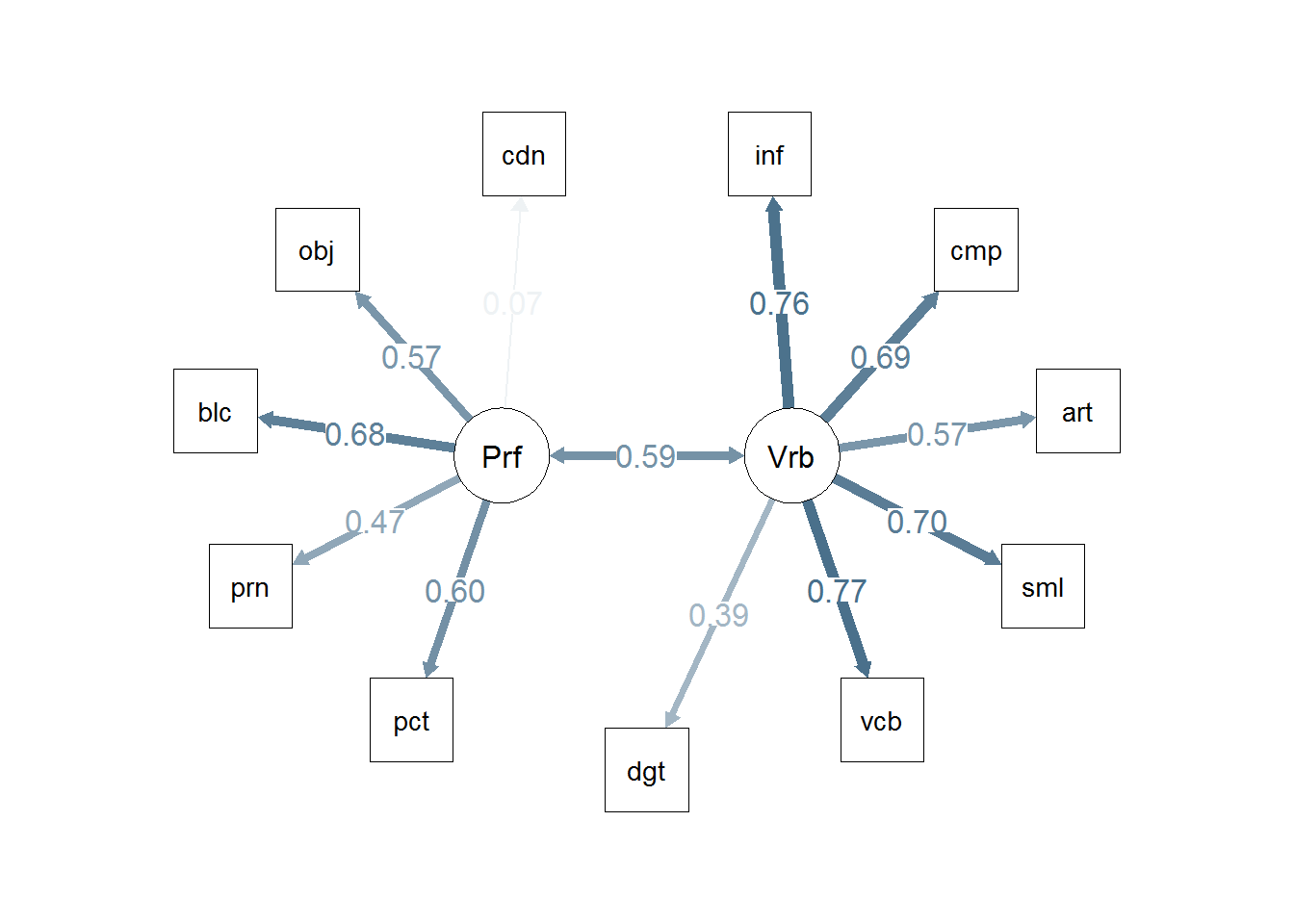
# or we could draw the paths in such a way to include the residuals:
#semPaths(m1, sizeMan=7,"std",edge.color="skyblue4",edge.label.cex=1,layout="circle2")
# the base path diagram can be drawn much more simply:
#semPaths(m1)
# or
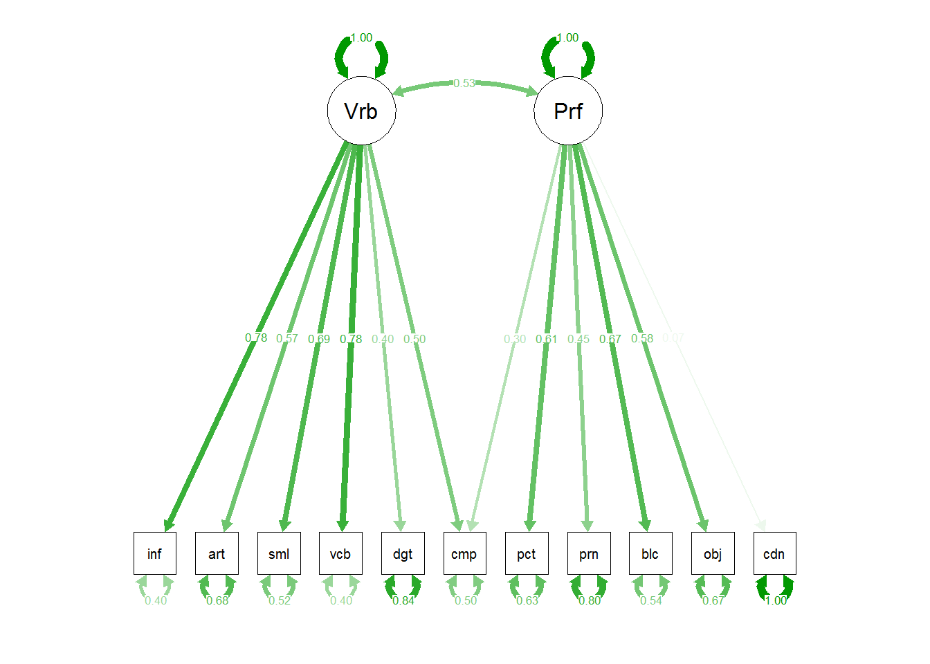
semPaths(m1,"std")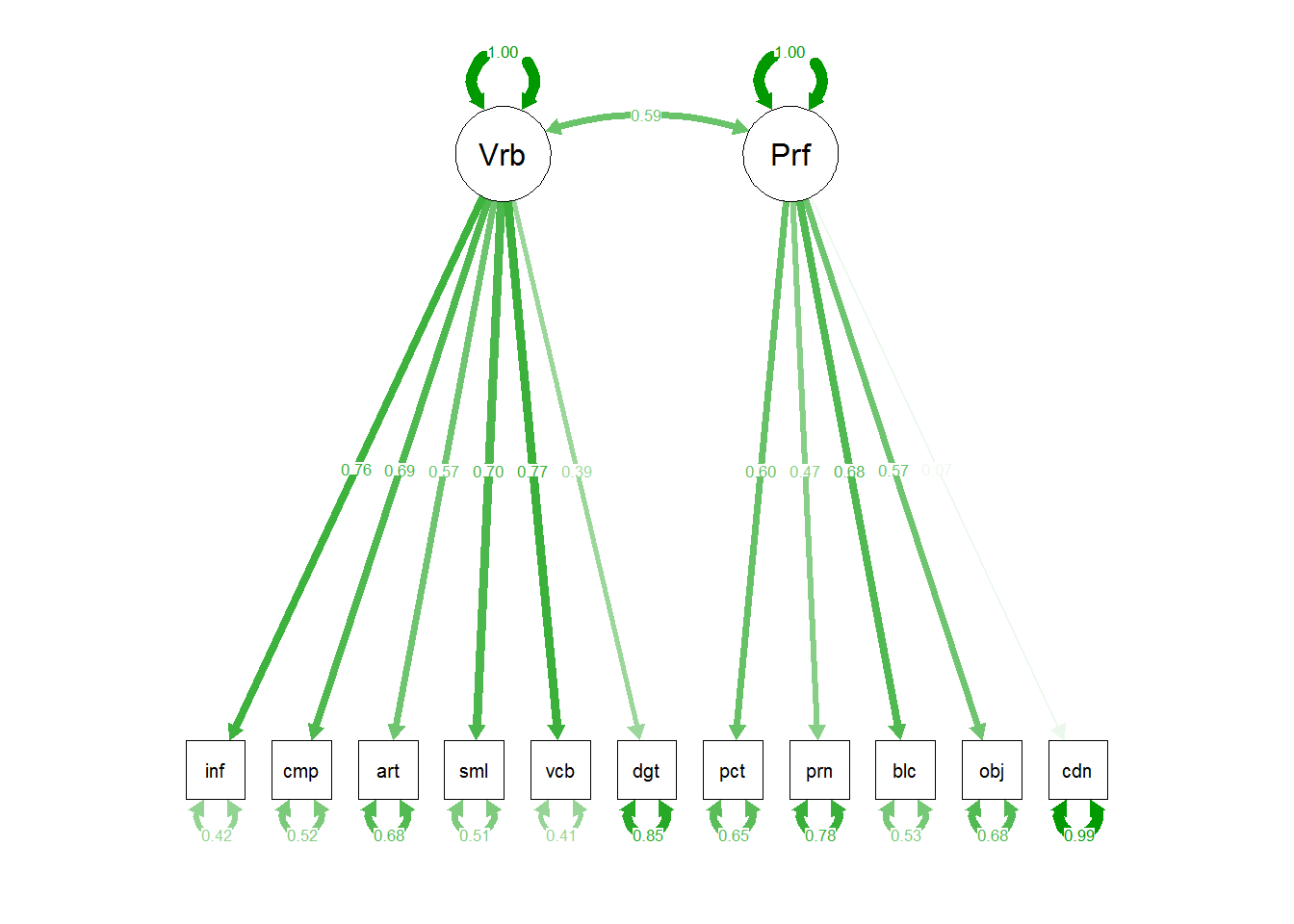
4.2 Example two
Model with added path still under construction in this chapter.
4.2.1 Define the second model
In the specifyModel text argument we just need to add one path, from Performance to “comp”, rerun the model, and compare to the first.
# this text could have been saved in a file and read in with the file argument to be efficient
# commented here to show the argument options
# m1.model <- specifyModel(file="sem2.txt")
m2.model <- specifyModel(text="
  ## Factor 1 is Verbal
  Verbal -> info, t01, NA
  Verbal -> comp, t02, NA
  Verbal -> arith, t03, NA
  Verbal -> simil, t04, NA
  Verbal -> vocab, t05, NA
  Verbal -> digit, t06, NA
  ## Factor 2 is performance
  Performance -> pictcomp, t07, NA
  Performance -> parang, t08, NA
  Performance -> block, t09, NA
  Performance -> object, t10, NA
  Performance -> coding, t11, NA
  Performance -> comp, t12, NA
  ## Set factor variances
  Verbal <-> Verbal, NA, 1
  Performance <-> Performance, NA, 1
  ## Set factor covariance to be estimable
  Verbal <-> Performance, p1, NA"
)
## NOTE: it is generally simpler to use specifyEquations() or cfa()
## see ?specifyEquations## NOTE: adding 11 variances to the model4.2.2 Fit model 2 and examine the results
In this chapter, we will just look at the basics of the model fit and draw the path diagram. Other aspects of the model can be extracted, but are passed over here to save space. The interested reader might try str(m1) to see what is available from the model object.
# all that is required is the model specification, the covariance matrix, and the sample size
m2 <- sem(m2.model,covwisc,175)
options(digits=5)
summary(m2)
##
## Model Chisquare = 60.295 Df = 42 Pr(>Chisq) = 0.033354
## AIC = 108.3
## BIC = -156.63
##
## Normalized Residuals
## Min. 1st Qu. Median Mean 3rd Qu. Max.
## -1.7087 -0.3670 0.0000 0.0439 0.4509 2.0855
##
## R-square for Endogenous Variables
## info comp arith simil vocab digit pictcomp parang
## 0.6036 0.5046 0.3227 0.4823 0.6044 0.1589 0.3741 0.2009
## block object coding
## 0.4551 0.3315 0.0049
##
## Parameter Estimates
## Estimate Std Error z value Pr(>|z|)
## t01 2.26254 0.200471 11.28609 1.5373e-29 info <--- Verbal
## t02 1.49558 0.255230 5.85973 4.6361e-09 comp <--- Verbal
## t03 1.31053 0.173300 7.56223 3.9620e-14 arith <--- Verbal
## t04 2.21107 0.227463 9.72056 2.4641e-22 simil <--- Verbal
## t05 2.28001 0.201829 11.29675 1.3616e-29 vocab <--- Verbal
## t06 1.07784 0.213286 5.05351 4.3377e-07 digit <--- Verbal
## t07 1.79476 0.240149 7.47352 7.8078e-14 pictcomp <--- Performance
## t08 1.19223 0.224879 5.30164 1.1477e-07 parang <--- Performance
## t09 1.82799 0.219975 8.30998 9.5719e-17 block <--- Performance
## t10 1.63752 0.234254 6.99037 2.7416e-12 object <--- Performance
## t11 0.20104 0.254172 0.79098 4.2896e-01 coding <--- Performance
## t12 0.88667 0.267519 3.31443 9.1829e-04 comp <--- Performance
## p1 0.53322 0.081099 6.57487 4.8695e-11 Performance <--> Verbal
## V[info] 3.36224 0.505946 6.64546 3.0227e-11 info <--> info
## V[comp] 4.35598 0.558735 7.79614 6.3830e-15 comp <--> comp
## V[arith] 3.60434 0.423598 8.50888 1.7563e-17 arith <--> arith
## V[simil] 5.24665 0.681040 7.70388 1.3199e-14 simil <--> simil
## V[vocab] 3.40241 0.512709 6.63614 3.2200e-11 vocab <--> vocab
## V[digit] 6.15077 0.682983 9.00574 2.1421e-19 digit <--> digit
## V[pictcomp] 5.38850 0.747358 7.21007 5.5922e-13 pictcomp <--> pictcomp
## V[parang] 5.65249 0.668468 8.45589 2.7697e-17 parang <--> parang
## V[block] 4.00164 0.628568 6.36628 1.9367e-10 block <--> block
## V[object] 5.40673 0.713201 7.58094 3.4306e-14 object <--> object
## V[coding] 8.20865 0.881648 9.31057 1.2715e-20 coding <--> coding
##
## Iterations = 37The table listing of parameter estimates uses the labeling strategy that was defined in the modelSpecify function. The names, such as theta01 are arbitrary.
4.2.3 Can we draw the path diagram from a sem model?
The semPaths function from semPlot is capable of recognizing a model object from sem. This code is identical to what was used in chapter 2 for the lavaan object. The fit object name is just changed to m2 here.
# Note that the base plot, including standardized path coefficients plots positive coefficients green
# and negative coefficients red.  Red-green colorblindness issues anyone?
# I redrew it here to choose a blue and red.  But all the coefficients in this example are
# positive,so they are shown with the skyblue.
# more challenging to use colors other than red and green.  not in this doc
semPaths(m2, residuals=F,sizeMan=7,"std",
         posCol=c("skyblue4", "red"),
         #edge.color="skyblue4",
         edge.label.cex=1.2,layout="circle2")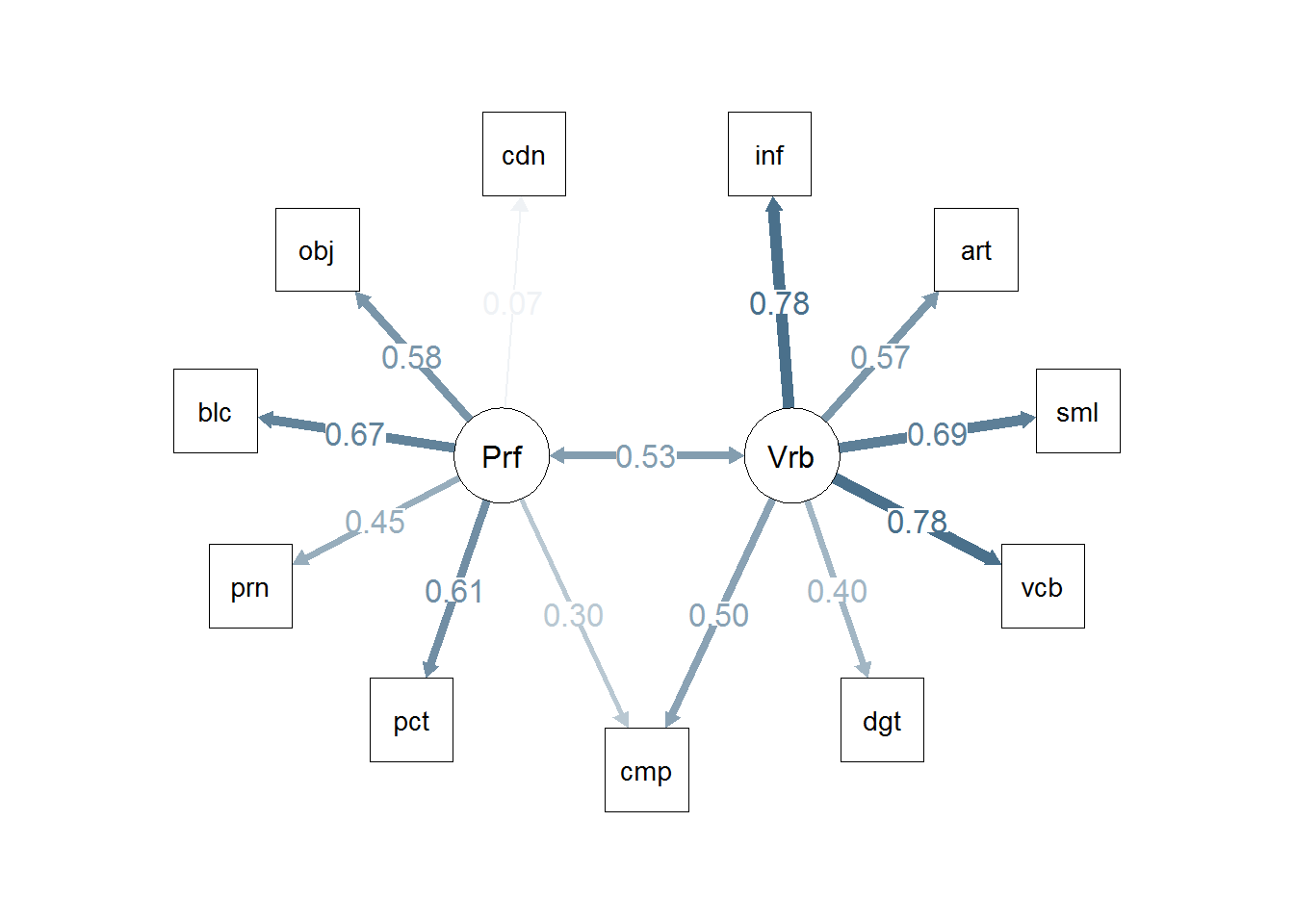
# or we could draw the paths in such  a way to include the residuals:
#semPaths(m1, sizeMan=7,"std",edge.color="skyblue4",edge.label.cex=1,layout="circle2")
# the base path diagram can be drawn much more simply:
#semPaths(m1)
# or
semPaths(m2,"std")