Chapter 5 Using the OpenMx Package for CFA
The OpenMX package in R is a port of the well-respected MX analytical software. It handles SEM and can easily be used for CFA. Here, the same two models that were run in lavaan will be run again, but an additional model will be run first.
5.1 First OpenMx Model - Single Factor
First, fit a bad model that posits only one underlying factor
5.1.2 Create the model using the mxModel function
This code initializes the model and sets vars/paths
latents="F1"
cfa2a <- mxModel("Common Factor Model",type="RAM",
                 manifestVars = manifests, latentVars = latents,
                 # Now set the residual variance for manifest variables
                 mxPath(from=manifests, arrows=2,free=T,values=1,labels=paste("error",1:11,sep="")),
                 # set latent factor variance to 1
                 mxPath(from="F1",arrows=2,free=F,values=1,labels="varF1"),
                 # specify factor loadings
                 mxPath(from="F1",to=manifests, arrows=1,
                        free=T,values=1,labels=paste("i", 1:11,sep="")),
                 # specify the covariance matrix
                 mxData(observed=observedCov,type="cov",numObs=numSubjects)
) # close the model
5.1.3 Now use mxRun to fit the model
mxRun uses the model defined above.
## Running Common Factor Model with 22 parametersSummarize the fit:
## Summary of Common Factor Model
##
## free parameters:
##       name matrix      row      col Estimate Std.Error A
## 1       i1      A     info       F1  2.10843   0.20493
## 2       i2      A     comp       F1  2.10259   0.20881
## 3       i3      A    arith       F1  1.27253   0.17312
## 4       i4      A    simil       F1  2.25978   0.22329
## 5       i5      A    vocab       F1  2.17498   0.20345
## 6       i6      A    digit       F1  1.00892   0.21304
## 7       i7      A pictcomp       F1  1.35055   0.22867
## 8       i8      A   parang       F1  0.89834   0.21225
## 9       i9      A    block       F1  1.23160   0.21129
## 10     i10      A   object       F1  1.01784   0.22713
## 11     i11      A   coding       F1  0.20128   0.23471
## 12  error1      S     info     info  3.98738   0.54530
## 13  error2      S     comp     comp  4.32199   0.56941
## 14  error3      S    arith    arith  3.67209   0.42699
## 15  error4      S    simil    simil  4.97099   0.64979
## 16  error5      S    vocab    vocab  3.82117   0.53016
## 17  error6      S    digit    digit  6.25281   0.68866
## 18  error7      S pictcomp pictcomp  6.73646   0.76231
## 19  error8      S   parang   parang  6.22646   0.68275
## 20  error9      S    block    block  5.78440   0.65292
## 21 error10      S   object   object  7.00600   0.77231
## 22 error11      S   coding   coding  8.16142   0.87321
##
## Model Statistics:
##                |  Parameters  |  Degrees of Freedom  |  Fit (-2lnL units)
##        Model:             22                     44                5492.0
##    Saturated:             66                      0                5375.1
## Independence:             11                     55                5894.3
## Number of observations/statistics: 175/66
##
## chi-square:  χ² ( df=44 ) = 116.85,  p = 1.5993e-08
## Information Criteria:
##       |  df Penalty  |  Parameters Penalty  |  Sample-Size Adjusted
## AIC:         28.851                 160.85                   167.51
## BIC:       -110.400                 230.48                   160.81
## CFI: 0.84306
## TLI: 0.80383   (also known as NNFI)
## RMSEA:  0.097268  [95% CI (0.071763, 0.12282)]
## Prob(RMSEA <= 0.05): 0.00026603
## timestamp: 2025-03-07 16:26:29
## Wall clock time: 0.040613 secs
## optimizer:  SLSQP
## OpenMx version number: 2.21.13
## Need help?  See help(mxSummary)
What is in the model?
## NULL## [1] "matrices" "algebras"
## [3] "data" "SaturatedLikelihood"
## [5] "IndependenceLikelihood" "calculatedHessian"
## [7] "vcov" "standardErrors"
## [9] "gradient" "hessian"
## [11] "expectations" "fit"
## [13] "fitUnits" "Minus2LogLikelihood"
## [15] "maxRelativeOrdinalError" "minimum"
## [17] "estimate" "infoDefinite"
## [19] "conditionNumber" "status"
## [21] "iterations" "evaluations"
## [23] "mxVersion" "frontendTime"
## [25] "backendTime" "independentTime"
## [27] "wallTime" "timestamp"
## [29] "cpuTime"5.2 Second OpenMx Model - the bifactor model
Now fit a model that is the same as the initial model fit with lavaan in chapter 3. Two factors, verbal and performance are established with each manifest variable uniquely specified by only one of the two latent factors.
5.2.2 Create the model using the mxModel function
Essentially initializes the model and sets vars/paths
cfa2b <- mxModel("Two Factor Model",type="RAM",
                 manifestVars = manifests, latentVars = latents2,
                 # Now set the residual variance for manifest variables
                 mxPath(from = manifests, arrows=2,free=T,values=1, labels=paste("e",1:11,sep="")),
                 # set latent factor variances
                 mxPath(from=latents2,arrows=2,free=F,values=1,labels=c("p1","p2")),
                 # speciffy factor loadings
                 # Allow the factors to covary as per the lavaan model
                 mxPath(from="verbal", to="perf", arrows=2,
                        free=T, values=1, labels="latcov1"),
                 # Specify the latent factor paths to manifests
                 mxPath(from="verbal", to = verbalVars,
                        arrows=1,
                        free=T,values=1),
                 mxPath(from="perf", to = perfVars,
                        arrows=1,
                        free=T,values=1),
                 mxData(observed=observedCov,type="cov",numObs=numSubjects)
) # close the model
5.2.3 Now use ’mxRun’to fit the model
mxRun uses the model defined above
## Running Two Factor Model with 23 parametersSummarize the fit
## Summary of Two Factor Model
##
## free parameters:
##                         name matrix      row      col Estimate Std.Error A
## 1   Two Factor Model.A[1,12]      A     info   verbal  2.20615  0.201343
## 2   Two Factor Model.A[2,12]      A     comp   verbal  2.04220  0.211972
## 3   Two Factor Model.A[3,12]      A    arith   verbal  1.29984  0.172691
## 4   Two Factor Model.A[4,12]      A    simil   verbal  2.23204  0.225255
## 5   Two Factor Model.A[5,12]      A    vocab   verbal  2.25045  0.200648
## 6   Two Factor Model.A[6,12]      A    digit   verbal  1.05277  0.212309 !
## 7   Two Factor Model.A[7,13]      A pictcomp     perf  1.74200  0.246159
## 8   Two Factor Model.A[8,13]      A   parang     perf  1.25323  0.224705
## 9   Two Factor Model.A[9,13]      A    block     perf  1.84593  0.224537
## 10 Two Factor Model.A[10,13]      A   object     perf  1.60457  0.236036
## 11 Two Factor Model.A[11,13]      A   coding     perf  0.20702  0.257070 !
## 12                        e1      S     info     info  3.56571  0.516714
## 13                        e2      S     comp     comp  4.57228  0.594754
## 14                        e3      S    arith    arith  3.60185  0.421970 !
## 15                        e4      S    simil    simil  5.09555  0.666227
## 16                        e5      S    vocab    vocab  3.48719  0.507522 !
## 17                        e6      S    digit    digit  6.16242  0.680927
## 18                        e7      S pictcomp pictcomp  5.52590  0.771998
## 19                        e8      S   parang   parang  5.46288  0.658748
## 20                        e9      S    block    block  3.89375  0.651513
## 21                       e10      S   object   object  5.46735  0.719615
## 22                       e11      S   coding   coding  8.15909  0.874167
## 23                   latcov1      S   verbal     perf  0.58884  0.077185
##
## Model Statistics:
##                |  Parameters  |  Degrees of Freedom  |  Fit (-2lnL units)
##        Model:             23                     43                5445.7
##    Saturated:             66                      0                5375.1
## Independence:             11                     55                5894.3
## Number of observations/statistics: 175/66
##
## chi-square:  χ² ( df=43 ) = 70.608,  p = 0.0050089
## Information Criteria:
##       |  df Penalty  |  Parameters Penalty  |  Sample-Size Adjusted
## AIC:        -15.392                 116.61                   123.92
## BIC:       -151.478                 189.40                   116.56
## CFI: 0.94053
## TLI: 0.92393   (also known as NNFI)
## RMSEA:  0.060571  [95% CI (0.026575, 0.089595)]
## Prob(RMSEA <= 0.05): 0.23348
## timestamp: 2025-03-07 16:26:30
## Wall clock time: 0.044815 secs
## optimizer:  SLSQP
## OpenMx version number: 2.21.13
## Need help?  See help(mxSummary)
What is in the model?
## NULL## [1] "matrices" "algebras"
## [3] "data" "SaturatedLikelihood"
## [5] "IndependenceLikelihood" "calculatedHessian"
## [7] "vcov" "standardErrors"
## [9] "gradient" "hessian"
## [11] "expectations" "fit"
## [13] "fitUnits" "Minus2LogLikelihood"
## [15] "maxRelativeOrdinalError" "minimum"
## [17] "estimate" "infoDefinite"
## [19] "conditionNumber" "status"
## [21] "iterations" "evaluations"
## [23] "mxVersion" "frontendTime"
## [25] "backendTime" "independentTime"
## [27] "wallTime" "timestamp"
## [29] "cpuTime"5.2.4 Can we use semPlot to draw the OpenMx model fit?
The semPlot package is very powerful and can recognize many lm and sem model objects. We can use the identical code that we used in chapter 2 for the lavaan model.
# Note that the base plot, including standardized path coefficients plots positive coefficients green
# and negative coefficients red.  Red-green colorblindness issues anyone?
# I redrew it here to choose a blue and red.  But all the coefficients in this example are
# positive,so they are shown with the skyblue.
# more challenging to use colors other than red and green.  not in this doc
semPaths(cfa2b, residuals=F,sizeMan=7,"std",
         posCol=c("skyblue4", "red"),
         #edge.color="skyblue4",
         edge.label.cex=1.2,layout="circle2")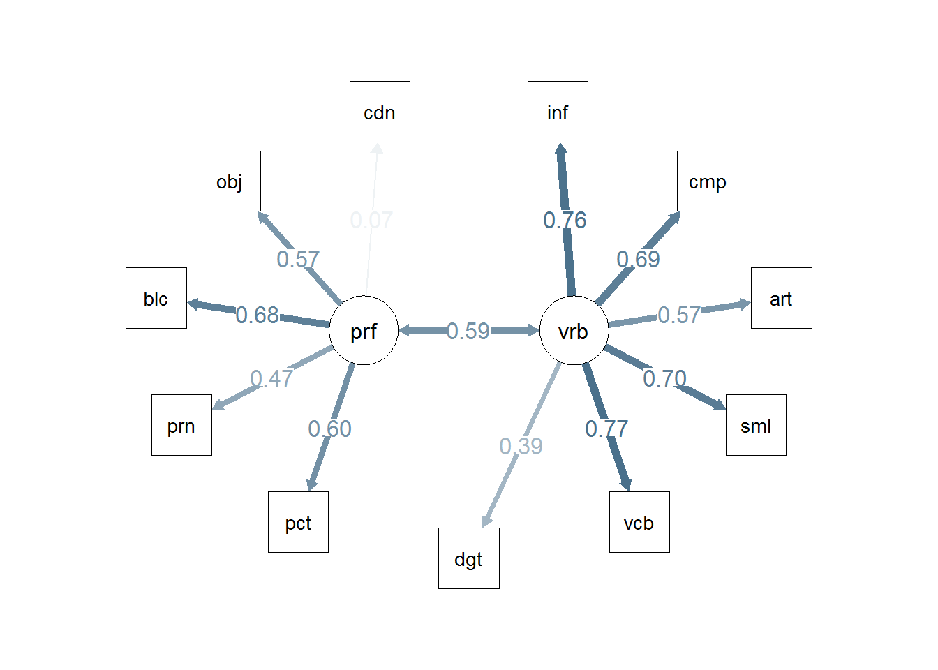
# or we could draw the paths in such  a way to include the residuals:
#semPaths(fit1, sizeMan=7,"std",edge.color="skyblue4",edge.label.cex=1,layout="circle2")
# the base path diagram can be drawn much more simply:
#semPaths(fit1)
# or
semPaths(cfa2b,"std")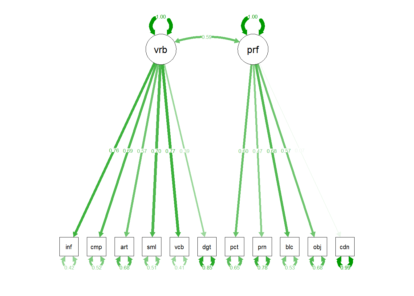
5.3 Third OpenMx Model
Now fit a model that is the same as the second model fit with lavaan above. Two factors, verbal and performance, plus paths from both latents to “comp”.
5.3.2 Create the model using the mxModel function
Essentially initializes the model and sets vars/paths
cfa2c <- mxModel("TwoFac, Comp Common",type="RAM",
                 manifestVars = manifests, latentVars = latents2,
                 # Now set the residual variance for manifest variables
                 mxPath(from = manifests, arrows=2,free=T,values=1, labels=paste("e",1:11,sep="")),
                 # set latent factor variances
                 mxPath(from=latents2,arrows=2,free=F,values=1,labels=c("p1","p2")),
                 # speciffy factor loadings
                 # Allow the factors to covary as per the lavaan model
                 mxPath(from="verbal", to="perf", arrows=2,
                        free=T, values=1, labels="latcov1"),
                 # Specify the latent factor paths to manifests
                 mxPath(from="verbal", to = verbalVars,
                        arrows=1,
                        free=T,values=1),
                 mxPath(from="perf", to = perfVars,
                        arrows=1,
                        free=T,values=1),
                 mxData(observed=observedCov,type="cov",numObs=numSubjects)
) # close the model
5.3.3 Now use ‘mxRun’ to fit the model
mxRun uses the model defined above
## Running TwoFac, Comp Common with 24 parametersSummarize the fit
## Summary of TwoFac, Comp Common
##
## free parameters:
##                            name matrix      row      col Estimate Std.Error A
## 1   TwoFac, Comp Common.A[1,12]      A     info   verbal  2.25606  0.200307
## 2   TwoFac, Comp Common.A[2,12]      A     comp   verbal  1.49129  0.256435 !
## 3   TwoFac, Comp Common.A[3,12]      A    arith   verbal  1.30679  0.173045
## 4   TwoFac, Comp Common.A[4,12]      A    simil   verbal  2.20475  0.227320
## 5   TwoFac, Comp Common.A[5,12]      A    vocab   verbal  2.27349  0.200587
## 6   TwoFac, Comp Common.A[6,12]      A    digit   verbal  1.07476  0.212337
## 7   TwoFac, Comp Common.A[2,13]      A     comp     perf  0.88415  0.270298
## 8   TwoFac, Comp Common.A[7,13]      A pictcomp     perf  1.78962  0.242398 !
## 9   TwoFac, Comp Common.A[8,13]      A   parang     perf  1.18883  0.225099 !
## 10  TwoFac, Comp Common.A[9,13]      A    block     perf  1.82277  0.221631 !
## 11 TwoFac, Comp Common.A[10,13]      A   object     perf  1.63283  0.233233 !
## 12 TwoFac, Comp Common.A[11,13]      A   coding     perf  0.20047  0.255206
## 13                           e1      S     info     info  3.34304  0.509424
## 14                           e2      S     comp     comp  4.33106  0.557290 !
## 15                           e3      S    arith    arith  3.58374  0.422014
## 16                           e4      S    simil    simil  5.21667  0.682623
## 17                           e5      S    vocab    vocab  3.38298  0.507439
## 18                           e6      S    digit    digit  6.11562  0.677540
## 19                           e7      S pictcomp pictcomp  5.35763  0.755723 !
## 20                           e8      S   parang   parang  5.62020  0.665632 !
## 21                           e9      S    block    block  3.97879  0.636699
## 22                          e10      S   object   object  5.37590  0.708176 !
## 23                          e11      S   coding   coding  8.16173  0.874162
## 24                      latcov1      S   verbal     perf  0.53322  0.082034 !
##
## Model Statistics:
##                |  Parameters  |  Degrees of Freedom  |  Fit (-2lnL units)
##        Model:             24                     42                5435.7
##    Saturated:             66                      0                5375.1
## Independence:             11                     55                5894.3
## Number of observations/statistics: 175/66
##
## chi-square:  χ² ( df=42 ) = 60.61,  p = 0.031396
## Information Criteria:
##       |  df Penalty  |  Parameters Penalty  |  Sample-Size Adjusted
## AIC:         -23.39                 108.61                   116.61
## BIC:        -156.31                 184.56                   108.56
## CFI: 0.95991
## TLI: 0.9475   (also known as NNFI)
## RMSEA:  0.050319  [95% CI (0, 0.081389)]
## Prob(RMSEA <= 0.05): 0.4664
## timestamp: 2025-03-07 16:26:33
## Wall clock time: 0.039705 secs
## optimizer:  SLSQP
## OpenMx version number: 2.21.13
## Need help?  See help(mxSummary)
What is in the model?
## NULL## [1] "matrices" "algebras"
## [3] "data" "SaturatedLikelihood"
## [5] "IndependenceLikelihood" "calculatedHessian"
## [7] "vcov" "standardErrors"
## [9] "gradient" "hessian"
## [11] "expectations" "fit"
## [13] "fitUnits" "Minus2LogLikelihood"
## [15] "maxRelativeOrdinalError" "minimum"
## [17] "estimate" "infoDefinite"
## [19] "conditionNumber" "status"
## [21] "iterations" "evaluations"
## [23] "mxVersion" "frontendTime"
## [25] "backendTime" "independentTime"
## [27] "wallTime" "timestamp"
## [29] "cpuTime"5.3.4 Draw the OpenMx model number 3
The semPlot package is very powerful and can recognize many ‘lm’ and SEM model objects. We can use the identical code that we used in chapter 2 for the lavaan model.
# Note that the base plot, including standardized path coefficients plots positive coefficients green
# and negative coefficients red.  Red-green colorblindness issues anyone?
# I redrew it here to choose a blue and red.  But all the coefficients in this example are
# positive,so they are shown with the skyblue.
# more challenging to use colors other than red and green.  not in this doc
semPaths(cfa2c, residuals=F,sizeMan=7,"std",
         posCol=c("skyblue4", "red"),
         #edge.color="skyblue4",
         edge.label.cex=1.2,layout="circle2")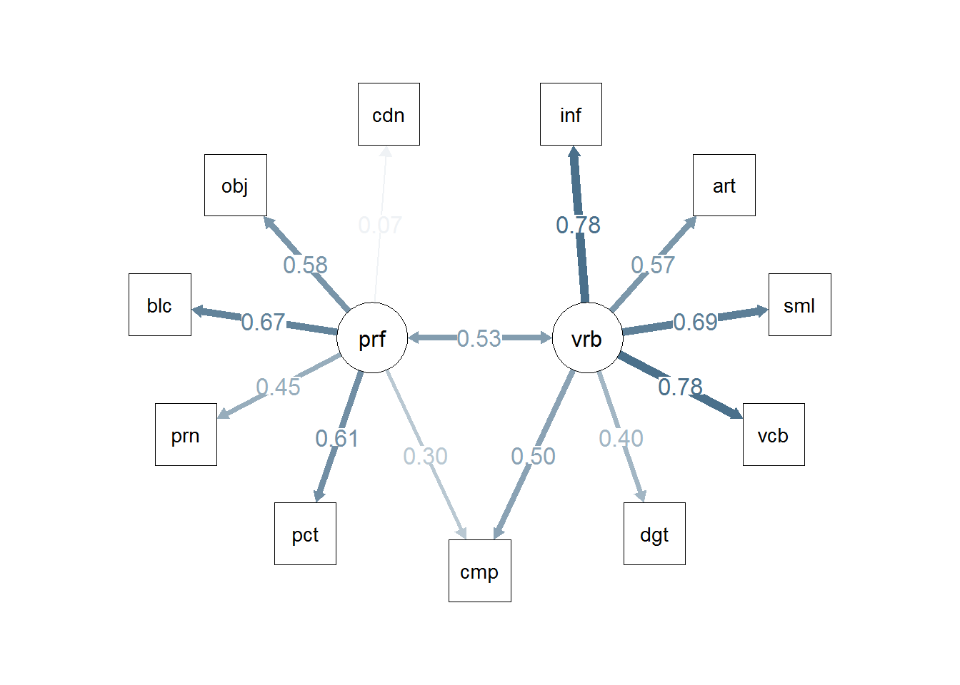
# or we could draw the paths in such  a way to include the residuals:
#semPaths(fit1, sizeMan=7,"std",edge.color="skyblue4",edge.label.cex=1,layout="circle2")
# the base path diagram can be drawn much more simply:
#semPaths(fit1)
# or
semPaths(cfa2c,"std")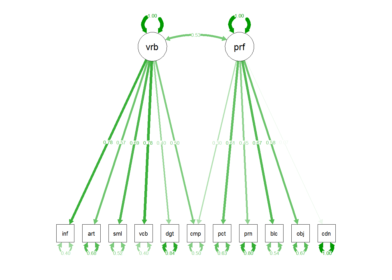
5.4 Compare the OpenMx models
In OpenMx a convenient function exists for model comparisons. This code compares the same two models that we initially compared in the lavaan approach that used the anova function.
| base | comparison | ep | minus2LL | df | AIC | diffLL | diffdf | p | fit | fitUnits | diffFit | chisq | SBchisq |
|---|---|---|---|---|---|---|---|---|---|---|---|---|---|
| TwoFac, Comp Common | NA | 24 | 5435.7 | 42 | 5483.7 | NA | NA | NA | 5435.7 | -2lnL | NA | NA | NA |
| TwoFac, Comp Common | Two Factor Model | 23 | 5445.7 | 43 | 5491.7 | 9.998 | 1 | 0.00157 | 5445.7 | -2lnL | 9.998 | NA | NA |