Chapter 4 Analytical Contrasts
Once first decision is made regarding univariate (the so-called averaged F test) vs multivariate tests, the user must still decide how to proceed in following up these omnibus tests with pairwise comparisons or analytical/orthogonal contrasts. It can be argued that the omnibus F tests in ANOVA are largely superfluous to the goals of researchers. Studies are designed with specific a priori hypotheses that should/could be specified as contrasts, including potential multi-group comparisons. This approach is viewed as more elegant and flexible that a shotgun approach of doing all pairwise comparisons among levels. Although assessment of pairwise comparisons among levels of a repeated measures factor are covered in this document, the analytical (and perhaps orthogonal) contrasts approach is considered the method of choice.
Until recently, and unfortunately, most of the built-in methods I have found employ the omnibus Axs error term in creating standard errors or F tests for such comparisons. This error term will almost always be flawed because of the likely lack of sphericity that is common in repeated measures studies. This is what we saw above in the attempt to use the “split” argument in the summary of the aov fit in the first part of this chapter.
The theory that outlines the rationale for specific error terms is summarized in the following figure which envisions partitioning the omnibus effect into contrasts and the Axs interaction into interaction contrasts which are the specific error terms for their respective contrast:
 These specific error terms are not flawed in the presence of non-sphericity. They can also be viewed as “tailored” to the contrast in question and may be generally preferred. In the rare circumstance where sphericity can be confidently assumed, then use of the omnibus error term would provide more power (larger df). Otherwise, specific error terms should be seen as the preferred approach.
We will see how use of the emmeans enables hypothesis tests with specific error terms, but only for some ANOVA fit objects. This is outlined in the section on afex and emmeans usage toward the end of this chapter.
It is possible to obtain specific error terms are with the manual approaches outlined below or perhaps in following up linear mixed effects modeling (next chapter). The manual approaches are not terribly burdensome for a simple one factor repeated measures design, but will become very much more challenging for larger designs - e.g., two repeated factors or mixed designs with grouping factors and repeated measures factors.
The conclusion I still hold is that the SPSS MANOVA procedure is efficient and helpful in pursuing these followup contrast types of questions. The SPSS GLM procedure can also be used, but its syntax (with L matrix specification) is obnoxiously obtuse. The default setting of specific error terms is of considerable value in the MANOVA procedure. It is not clear to me why this has not found its way into the R ecosystem more prominently. It is perhaps because the standard data format for repeated measures is the long format data structure. Specific error terms are more easily generated out of wide format data structures, for repeated measures. Perhaps there is still something I haven’t yet learned about the suite of R functions available. Or see the use of the glht function usage in the last sections in the next chapter here.
4.1 Partitioning the omnibus effect into orthogonal contrasts
The value of full rank models that employ orthogonal contrast sets is clear for completely randomized designs (between-groups designs). For repeated measures factors partitioning into orthogonal sets is useful for establishing the Omnibus F test of the factor as well. Non-orthogonal contrasts with alpha rate adjustments can also be useful and attention that that approach is possible with the emmeans function later in this chapter and the glht function in the next chapter.
4.2 Contrasts with the aov model object
Rather than use the default indicator coding or the “contr.sum” coding that was used initially, we can change the contrasts for the repeated measure factor using the same approach considered for between subjects factors in completely randomized designs. The set chosen here would likely contain several a priori hypotheses about this design and all four contrasts are rational.
contrasts.type <- matrix(c(4, -1, -1, -1, -1,
                           0,  3, -1, -1, -1,
                           0,  0, -1, -1,  2,
                           0,  0, -1,  1,  0),
                           ncol=4)
contrasts(rpt1.df$type) <- contrasts.type
contrasts(rpt1.df$type)
## [,1] [,2] [,3] [,4]
## clean 4 0 0 0
## homecage -1 3 0 0
## iguana -1 -1 -1 -1
## whiptail -1 -1 -1 1
## krat -1 -1 2 0Once this set is in place, we can use familiar methods for finding tests of these contrasts. The same aov model fit that comprised Method I above is implemented again here. In a second application of the summary function to the aov model object, we can use the “split” argument to obtain evaluation of these four orthogonal contrasts.
From examination of the four F values and their component numerator and denominator MS, we can see that these four tests all use the OMNIBUS error term and are not GG/HF adjusted. Specific error terms are, unfortunately, not possible using the aov function for the model fit. The summary.lm function also will not work with a repeated measures object fit from aov. Other methods for obtaining evaluation of contrasts are found below.
fit.1 <- aov(DV~type + Error(snum/type), data=rpt1.df)
summary(fit.1)
##
## Error: snum
## Df Sum Sq Mean Sq F value Pr(>F)
## Residuals 9 3740 415.5
##
## Error: snum:type
## Df Sum Sq Mean Sq F value Pr(>F)
## type 4 2042 510.4 8.845 4.42e-05 ***
## Residuals 36 2077 57.7
## ---
## Signif. codes: 0 '***' 0.001 '**' 0.01 '*' 0.05 '.' 0.1 ' ' 1summary(fit.1, split=list(type=list(ac1=1, ac2=2, ac3=3, ac4=4)))##
## Error: snum
## Df Sum Sq Mean Sq F value Pr(>F)
## Residuals 9 3740 415.5
##
## Error: snum:type
## Df Sum Sq Mean Sq F value Pr(>F)
## type 4 2041.5 510.4 8.845 4.42e-05 ***
## type: ac1 1 173.0 173.0 2.998 0.0919 .
## type: ac2 1 396.0 396.0 6.863 0.0128 *
## type: ac3 1 1450.4 1450.4 25.136 1.44e-05 ***
## type: ac4 1 22.1 22.1 0.382 0.5404
## Residuals 36 2077.3 57.7
## ---
## Signif. codes: 0 '***' 0.001 '**' 0.01 '*' 0.05 '.' 0.1 ' ' 14.3 Contrasts with the Method III “mlmfit” object
We saw in the earlier chapter that contrast SS could be obtained from the “mlmfit” approach. Since orthogonal polynomial trend analysis, as done in the initial Method III analysis, is not appropriate for our “stimulus/type” factor, next we can add in the ability to specify our own contrasts. This is the same orthogonal set used just above. The name of the factor was changed to “stimulus” for this approach so as to not confuse it with the aov approach where we used the variable name “type” in the long format data frame. Then we will rerun the Anova function from car, using these contrasts.
contrasts.stimulus <- matrix(c(4, -1, -1, -1, -1,
                               0,  3, -1, -1, -1,
                               0,  0, -1, -1,  2,
                               0,  0, -1,  1,  0),
                             ncol=4)
contrasts(stimulus) <- contrasts.stimulus
contrasts(stimulus)
## [,1] [,2] [,3] [,4]
## clean 4 0 0 0
## homecage -1 3 0 0
## iguana -1 -1 -1 -1
## whiptail -1 -1 -1 1
## krat -1 -1 2 0icontr <- contrasts(stimulus)First we will refit the same “mlmfit” model as from Method III in the earlier chapter.
# start by defining the multivariate linear model
# this code returns the level means.
mlmfit.2 <- lm(rpt1w.mat ~1)
mlmfit.2
##
## Call:
## lm(formula = rpt1w.mat ~ 1)
##
## Coefficients:
## clean homecage iguana whiptail krat
## (Intercept) 6.8 6.0 7.3 9.4 23.1Next we redo the application of the Anova function to that model fit with an additional specification. The new “icontr” object is specified with one additional argument in Anova, called “icontrasts”.
Also notice:
Hypothesis SS and for each contrast are produced, but only found in the SSP matrix and t/F tests not performed. We will have to compute the F’s manually after computing the respective MS.
The error SS are computed for the contrasts but not printed by use of the
summaryfunction. We will have to manually extract them.The hypothesis SS and error SS are not corrected for the size of the coefficients chosen. I.e., the coefficients are not orthonormalized in this illustration, so the SS won’t match your SPSS-generated SS unless you divide each by the respective sum of the squared contrast coefficients.
Despite using the contrasts that we specified,
Anovadoes not produce tests of those individual contrasts with thesummaryfunction. I have not found a direct way to obtain those tests. In the next sections, I show ways to obtain them more “manually”
mlmfit3.anova <- Anova(mlmfit.2,
                       idata=data.frame(stimulus),
                       idesign=~stimulus,
                       icontrasts=icontr,type="III")
#str(mlmfit3.anova)
summary(mlmfit3.anova)
##
## Type III Repeated Measures MANOVA Tests:
##
## ------------------------------------------
##
## Term: (Intercept)
##
## Response transformation matrix:
## (Intercept)
## clean 1
## homecage 1
## iguana 1
## whiptail 1
## krat 1
##
## Sum of squares and products for the hypothesis:
## (Intercept)
## (Intercept) 27667.6
##
## Multivariate Tests: (Intercept)
## Df test stat approx F num Df den Df Pr(>F)
## Pillai 1 0.5967217 13.3171 1 9 0.0053237 **
## Wilks 1 0.4032783 13.3171 1 9 0.0053237 **
## Hotelling-Lawley 1 1.4796774 13.3171 1 9 0.0053237 **
## Roy 1 1.4796774 13.3171 1 9 0.0053237 **
## ---
## Signif. codes: 0 '***' 0.001 '**' 0.01 '*' 0.05 '.' 0.1 ' ' 1
##
## ------------------------------------------
##
## Term: stimulus
##
## Response transformation matrix:
## stimulus1 stimulus2 stimulus3 stimulus4
## clean 4 0 0 0
## homecage -1 3 0 0
## iguana -1 -1 -1 -1
## whiptail -1 -1 -1 1
## krat -1 -1 2 0
##
## Sum of squares and products for the hypothesis:
## stimulus1 stimulus2 stimulus3 stimulus4
## stimulus1 3459.6 4054.8 -5487.0 -390.6
## stimulus2 4054.8 4752.4 -6431.0 -457.8
## stimulus3 -5487.0 -6431.0 8702.5 619.5
## stimulus4 -390.6 -457.8 619.5 44.1
##
## Multivariate Tests: stimulus
## Df test stat approx F num Df den Df Pr(>F)
## Pillai 1 0.6495405 2.780095 4 6 0.12692
## Wilks 1 0.3504595 2.780095 4 6 0.12692
## Hotelling-Lawley 1 1.8533965 2.780095 4 6 0.12692
## Roy 1 1.8533965 2.780095 4 6 0.12692
##
## Univariate Type III Repeated-Measures ANOVA Assuming Sphericity
##
## Sum Sq num Df Error SS den Df F value Pr(>F)
## (Intercept) 5533.5 1 3739.7 9 13.3171 0.005324 **
## stimulus 2041.5 4 2077.3 36 8.8447 4.424e-05 ***
## ---
## Signif. codes: 0 '***' 0.001 '**' 0.01 '*' 0.05 '.' 0.1 ' ' 1
##
##
## Mauchly Tests for Sphericity
##
## Test statistic p-value
## stimulus 0.0038542 7.3907e-06
##
##
## Greenhouse-Geisser and Huynh-Feldt Corrections
## for Departure from Sphericity
##
## GG eps Pr(>F[GG])
## stimulus 0.3793 0.005501 **
## ---
## Signif. codes: 0 '***' 0.001 '**' 0.01 '*' 0.05 '.' 0.1 ' ' 1
##
## HF eps Pr(>F[HF])
## stimulus 0.4400688 0.003391046The omnibus univariate and multivariate tests are identical the the initial Method III illustration above. Unfortunately, there does not appear to be a way of requesting that Anova test these newly created contrasts.
The output just above did give the SS for each of the contrasts, seen on the leading diagonal of the SSP (hypothesis matrix). The Anova function did create the error SS as well, but they were not printed with the results. In order to find the error SS for each contrast (the Acontrast x s) terms for specific error terms, we need to examine the structure of the mlmfit3.anova object. It is called the SSPE matrix. Note that in addition to the SShypothesis and SSerror values, we can look for the error df as well (it is called error.df)
str(mlmfit3.anova)## List of 14
## $ SSP :List of 2
## ..$ (Intercept): num [1, 1] 27668
## .. ..- attr(*, "dimnames")=List of 2
## .. .. ..$ : chr "(Intercept)"
## .. .. ..$ : chr "(Intercept)"
## ..$ stimulus : num [1:4, 1:4] 3460 4055 -5487 -391 4055 ...
## .. ..- attr(*, "dimnames")=List of 2
## .. .. ..$ : chr [1:4] "stimulus1" "stimulus2" "stimulus3" "stimulus4"
## .. .. ..$ : chr [1:4] "stimulus1" "stimulus2" "stimulus3" "stimulus4"
## $ SSPE :List of 2
## ..$ (Intercept): num [1, 1] 18698
## .. ..- attr(*, "dimnames")=List of 2
## .. .. ..$ : chr "(Intercept)"
## .. .. ..$ : chr "(Intercept)"
## ..$ stimulus : num [1:4, 1:4] 4976 4381 -5133 -169 4381 ...
## .. ..- attr(*, "dimnames")=List of 2
## .. .. ..$ : chr [1:4] "stimulus1" "stimulus2" "stimulus3" "stimulus4"
## .. .. ..$ : chr [1:4] "stimulus1" "stimulus2" "stimulus3" "stimulus4"
## $ P :List of 2
## ..$ (Intercept): num [1:5, 1] 1 1 1 1 1
## .. ..- attr(*, "dimnames")=List of 2
## .. .. ..$ : chr [1:5] "clean" "homecage" "iguana" "whiptail" ...
## .. .. ..$ : chr "(Intercept)"
## ..$ stimulus : num [1:5, 1:4] 4 -1 -1 -1 -1 0 3 -1 -1 -1 ...
## .. ..- attr(*, "dimnames")=List of 2
## .. .. ..$ : chr [1:5] "clean" "homecage" "iguana" "whiptail" ...
## .. .. ..$ : chr [1:4] "stimulus1" "stimulus2" "stimulus3" "stimulus4"
## $ df : Named num [1:2] 1 1
## ..- attr(*, "names")= chr [1:2] "(Intercept)" "stimulus"
## $ error.df : int 9
## $ terms : chr [1:2] "(Intercept)" "stimulus"
## $ repeated : logi TRUE
## $ type : chr "III"
## $ test : chr "Pillai"
## $ idata :'data.frame': 5 obs. of 1 variable:
## ..$ stimulus: Ord.factor w/ 5 levels "clean"<"homecage"<..: 1 2 3 4 5
## .. ..- attr(*, "contrasts")= num [1:5, 1:4] 4 -1 -1 -1 -1 0 3 -1 -1 -1 ...
## .. .. ..- attr(*, "dimnames")=List of 2
## .. .. .. ..$ : chr [1:5] "clean" "homecage" "iguana" "whiptail" ...
## .. .. .. ..$ : NULL
## $ idesign :Class 'formula' language ~stimulus
## .. ..- attr(*, ".Environment")=<environment: R_GlobalEnv>
## $ icontrasts: num [1:5, 1:4] 4 -1 -1 -1 -1 0 3 -1 -1 -1 ...
## ..- attr(*, "dimnames")=List of 2
## .. ..$ : chr [1:5] "clean" "homecage" "iguana" "whiptail" ...
## .. ..$ : NULL
## $ imatrix : NULL
## $ singular : Named logi [1:2] FALSE FALSE
## ..- attr(*, "names")= chr [1:2] "(Intercept)" "stimulus"
## - attr(*, "class")= chr "Anova.mlm"This SSP matrix duplicates the information that was seen in the summary output and the SS for the contrasts are on the leading diagonal. They are numerically larger than those from the summary output above, but by the expected factor of the sum of the squared coefficients for each contrast - they are not orthonormalized.
# view the contrast hypothesis SS_CP matrix
mlmfit3.anova$SSP$stimulus
## stimulus1 stimulus2 stimulus3 stimulus4
## stimulus1 3459.6 4054.8 -5487.0 -390.6
## stimulus2 4054.8 4752.4 -6431.0 -457.8
## stimulus3 -5487.0 -6431.0 8702.5 619.5
## stimulus4 -390.6 -457.8 619.5 44.1Similarly, the SS for the specific errors are found on the leading diagonal of this SSPE matrix - again, not orthonormalized contrasts.
# view the contrast error SS_CP matrix
mlmfit3.anova$SSPE$stimulus
## stimulus1 stimulus2 stimulus3 stimulus4
## stimulus1 4976.4 4381.2 -5133.0 -169.4
## stimulus2 4381.2 6371.6 -4069.0 369.8
## stimulus3 -5133.0 -4069.0 6882.5 735.5
## stimulus4 -169.4 369.8 735.5 300.9In order to do the F tests, we need to:
- Extract the relevant SS from the leading diagonals of the matrices examined above.
- Create the MS error for each contrast by dividing by the correct df for the Axs term (1x(s-1))
- Realize that each contrast is a 1df source, so each hypothesis SS is already a MS
- Divide the MSeffect values by the MSerror values to produce the F values
- find p values for each F
It made the naming easier to “attach” the mlmfit3.anova object. First, obtain the SSeffect values (equivalent to the MSeffect values since they are 1 df terms:
attach(mlmfit3.anova)
#show effect/cov values - the SS of the contrasts are on the diagonal
#SSP$stimulus
effect <- diag(SSP$stimulus)
#note that the diagonal from SSP matrix is already the MS since df = 1
effect
## stimulus1 stimulus2 stimulus3 stimulus4
## 3459.6 4752.4 8702.5 44.1Then obtain the MSerror values:
#show error/cov values - the specific error SS are on the diagonal
#SSPE$stimulus
x1 <- diag(SSPE$stimulus)
x1
## stimulus1 stimulus2 stimulus3 stimulus4
## 4976.4 6371.6 6882.5 300.9error <- x1/error.dfNow compute the F values and obtain p values for each contrast. Note that they match our SPSS work.
# now compute F's; F values are on the diagonal
Fvalues <- effect/error
Fvalues
## stimulus1 stimulus2 stimulus3 stimulus4
## 6.256812 6.712851 11.379949 1.319043# obtain the p values for the four F tests (all have 1,9 df)
pf(Fvalues,1,9,lower.tail=F)## stimulus1 stimulus2 stimulus3 stimulus4
## 0.033786236 0.029169567 0.008212304 0.280372227Once again, note that the MS values for the numerator and denominator are neither one corrected for the size of the coefficients chosen. But since neither are corrected, their ratio still produces the expected F value. We could have done more work to divide each SS first by the sum of the squared coefficients for each contrast, but the same F values would have been produced.
There is a more efficient way of doing this by writing a function and then passing the Anova object to it. F values and p values are returned.
model <- mlmfit3.anova
rptcontr <- function(model){
  SSCPeffect <- as.matrix(model$SSP$stimulus,ncol=4)
  effect <- diag(SSCPeffect)
  #effect
  #return(effect)
  SSCPerror <- as.matrix(model$SSPE$stimulus,ncol=4)
  error <- diag(SSCPerror)
  dferror <- mlmfit3.anova$error.df
  mserror <- error/dferror
  Fval <- round(effect/mserror,3)
  pval <- round(pf(Fval, 1,dferror, lower.tail=F),4)
  vals <- as.data.frame(cbind(Fval, pval, dferror))
  vals
  return(gt(vals,rownames_to_stub=T))
}
rptcontr(model=mlmfit3.anova)| Fval | pval | dferror | |
|---|---|---|---|
| stimulus1 | 6.257 | 0.0338 | 9 |
| stimulus2 | 6.713 | 0.0292 | 9 |
| stimulus3 | 11.380 | 0.0082 | 9 |
| stimulus4 | 1.319 | 0.2804 | 9 |
4.4 Recall how to “manually” implement contrasts for repeated factors.
The method for obtaining contrasts just reviewed is very laborious and does not easily extend to multiple factor repeated measures designs. At this point, it would be useful to recall another class demonstration of how to conceptualize contrasts for repeated measures.
Since each case provides a data point for each level of the repeated measure factor, we can create contrast vectors manually as new variables - essentially transformations. I have used the mutate function from dplyr to do this. For a review of mutate, see the separate document on subsetting and variable creation.
rpt1w.df <- mutate(rpt1w.df,
            ac1=(4*clean+(-1)*homecage+(-1)*iguana+(-1)*whiptail+(-1)*krat))
rpt1w.df <- mutate(rpt1w.df,
            ac2=(0*clean+(3)*homecage+(-1)*iguana+(-1)*whiptail+(-1)*krat))
rpt1w.df <- mutate(rpt1w.df,
            ac3=(0*clean+(0)*homecage+(-1)*iguana+(-1)*whiptail+(2)*krat))
rpt1w.df <- mutate(rpt1w.df,
            ac4=(0*clean +(0)*homecage+(-1)*iguana+(1)*whiptail+(0)*krat))
gt(rpt1w.df)| snum | clean | homecage | iguana | whiptail | krat | ac1 | ac2 | ac3 | ac4 |
|---|---|---|---|---|---|---|---|---|---|
| 1 | 24 | 15 | 41 | 30 | 50 | -40 | -76 | 29 | -11 |
| 2 | 6 | 6 | 0 | 6 | 13 | -1 | -1 | 20 | 6 |
| 3 | 4 | 0 | 5 | 4 | 9 | -2 | -18 | 9 | -1 |
| 4 | 11 | 9 | 10 | 14 | 18 | -7 | -15 | 12 | 4 |
| 5 | 0 | 0 | 0 | 0 | 0 | 0 | 0 | 0 | 0 |
| 6 | 8 | 15 | 10 | 15 | 38 | -46 | -18 | 51 | 5 |
| 7 | 8 | 5 | 2 | 6 | 15 | 4 | -8 | 22 | 4 |
| 8 | 0 | 0 | 0 | 11 | 54 | -65 | -65 | 97 | 11 |
| 9 | 0 | 3 | 1 | 1 | 11 | -16 | -4 | 20 | 0 |
| 10 | 7 | 7 | 4 | 7 | 23 | -13 | -13 | 35 | 3 |
Once created, we can test a hypothesis that each contrast has a value of zero (the null). Each contrast is now a single vector of ten values, and the sd of each vector is the square root of the specific error term MS values calculated above. So, when we perform a one sample t-test with a null value of zero, the t’s that are produced are the square roots of the F values computed above. One might compare the mean of the first contrast vector to the value we examined when we manually did this exercise in spreadsheet form at the point in time that the repeated measures theory was first presented in class.
Also note that these F’s (and the squares of the t’s below) do not match the F tests of these same contrasts that were obtained in the first section of this chapter where the “split” argument was used in the summary function. This is because the “split” approach uses the omnibus error term (MS Axs) for all of the contrasts, but the approaches here utilize error that is specific to each contrast. The latter would always be preferred when sphericity is not present in the data system (almost always).
t.test(rpt1w.df$ac1)##
## One Sample t-test
##
## data: rpt1w.df$ac1
## t = -2.5014, df = 9, p-value = 0.03379
## alternative hypothesis: true mean is not equal to 0
## 95 percent confidence interval:
## -35.421285 -1.778715
## sample estimates:
## mean of x
## -18.6t.test(rpt1w.df$ac2)##
## One Sample t-test
##
## data: rpt1w.df$ac2
## t = -2.5909, df = 9, p-value = 0.02917
## alternative hypothesis: true mean is not equal to 0
## 95 percent confidence interval:
## -40.833812 -2.766188
## sample estimates:
## mean of x
## -21.8t.test(rpt1w.df$ac3)##
## One Sample t-test
##
## data: rpt1w.df$ac3
## t = 3.3734, df = 9, p-value = 0.008212
## alternative hypothesis: true mean is not equal to 0
## 95 percent confidence interval:
## 9.717798 49.282202
## sample estimates:
## mean of x
## 29.5t.test(rpt1w.df$ac4)##
## One Sample t-test
##
## data: rpt1w.df$ac4
## t = 1.1485, df = 9, p-value = 0.2804
## alternative hypothesis: true mean is not equal to 0
## 95 percent confidence interval:
## -2.036306 6.236306
## sample estimates:
## mean of x
## 2.1This manual approach works well, is fairly efficient, and is important because of its use of the error terms specific to the contrast rather than the omnibus Axs error term which is burdened with the sphericity assumption. There is a literature that argues for the use of specific error terms to avoid this non-sphericity problem. Using the omnibus Axs error term may inflate type I error rates more for contrasts than for the omnibus F test in repeated measures designs when the sphericity assumption is violated (see section in the tookit bibliography, in particular a paper by Boik (Boik, 1981).
Also see chapter nine for a more efficient way of producing these specific error term approaches.
4.4.1 Create a plot of these contrasts and their specific errors
Modeling on the approach shown in chapter 2 for visualizing the pairwise comparisons, we plot the four orthogonal contrast means and standard errors for the contrasts just examined above with the one-sample t-test procedure. First we need to extract the variables from the wide format data frame and restructure the data to a long format. Then the summarySE function can be used to find the means, SE’s and CI’s.
aclong <-
  tidyr::pivot_longer(data=rpt1w.df[, c(1,7:10)],
                      cols=2:5,
                      names_to="contrast",
                      values_to="contrastvalue")
aclong
## # A tibble: 40 × 3
## snum contrast contrastvalue
## <int> <chr> <dbl>
## 1 1 ac1 -40
## 2 1 ac2 -76
## 3 1 ac3 29
## 4 1 ac4 -11
## 5 2 ac1 -1
## 6 2 ac2 -1
## 7 2 ac3 20
## 8 2 ac4 6
## 9 3 ac1 -2
## 10 3 ac2 -18
## # … with 30 more rowssummary.contrasts <- Rmisc::summarySE(aclong,
measurevar="contrastvalue",
groupvars="contrast")
summary.contrasts## contrast N contrastvalue sd se ci
## 1 ac1 10 -18.6 23.514535 7.435949 16.821285
## 2 ac2 10 -21.8 26.607434 8.414009 19.033812
## 3 ac3 10 29.5 27.653611 8.744840 19.782202
## 4 ac4 10 2.1 5.782156 1.828478 4.136306Much like the plot of paired differences in chapter 2, the visual task here is to compare each mean value to zero. Confidence intervals are overlaid and we see all but the last contrast have CI’s that do not overlap zero, and that is what is expected since the first three were significant when tested above with the one-sample t-tests. The important point here is that the standard error used in calculating the CI is an error specific to the particular contrast.
Also note that contrast 4 is a pairwise comparison of the same pair of levels examined in chapter 2 as pair 4 and 3 (comparing whiptail lizard to iguana). The mean value, the CI, and the plot are the same here as for that pair seen in chapter 2.
This graph, plus the graph from chapter 2 of means plus raw data points would be a valueable way to present data for this design.
p10 <- ggplot(summary.contrasts, aes(x=contrast, y=contrastvalue, fill=contrast)) +
  geom_bar(position=position_dodge(), stat="identity", fill="gray") +
  geom_errorbar(aes(ymin=contrastvalue-ci, ymax=contrastvalue+ci), data=summary.contrasts,
                width=.2,                    # Width of the error bars
                position=position_dodge(.9)) +
  ggtitle("Means plus 95% CIs for Four Orthogonal Contrasts") +
  guides(fill=FALSE) + # removes legend
  theme_minimal() +
  theme(plot.title = element_text(size=10,
                                  face = "bold", hjust = .5))
p10 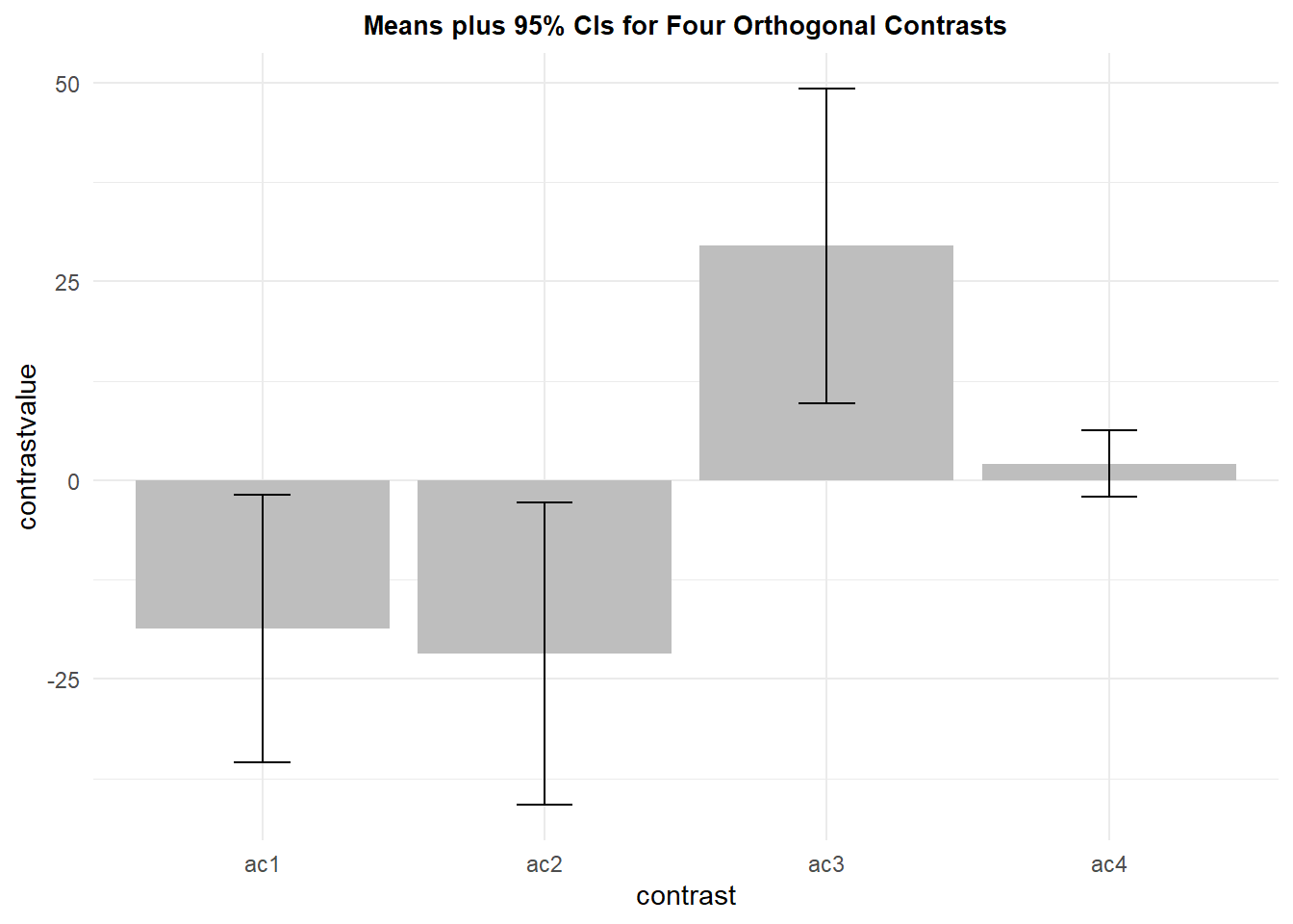
4.5 Working with afex and emmeans for contrasts and pairwise comparison follow ups
The emmeans package provides strong facilities for performing follow up analyses such as pairwise multiple comparisons and contrasts, in conjunction with an afex model. This section briefly demonstrates both of those. In a recent release of emmeans, the tests of contrasts and pairwise comparisons in this repeated measures design began to employ specific error terms instead of the flawed omnibus error term previously used. This may have resulted from a change in the aov_car function in afex to use a “multivariate/wide data” approach. For this 1 factor repeated measures design, emmeans can now be recommended, but only in conjunction wth an afex fit object. emmeans will not produce specific error terms when applied to aov models.
The emmeans function can utilize anova objects from a variety of sources. It works well with objects from afex so that is the approach taken here. The first line of code here simply extracts the information from the afex object to perform pairwise tests of the means of the five conditions. Since this would likely be a post hoc approach, the “adjust” argument in the “pairs” function permits access to the large family of correction types for error rate inflation. I illustrated the use with the Tukey method, but holm, by, bonf, fdr, and others are available. The df for the error in each of these tests is listed as 9 and the SE vary from test to test. This implies that the specific errors are used for all of the pairwise tests and that error is based on the potentially flawed MS Axs error term is avoided. The second pairs function here produces the same tests, but without p value adjustments.
fit1afex.emm <- emmeans(fit1.afex, "type", data=rpt1.df)
pairs(fit1afex.emm, adjust="tukey")
## contrast estimate SE df t.ratio p.value
## clean - homecage 0.8 1.34 9 0.597 0.9721
## clean - iguana -0.5 2.04 9 -0.245 0.9990
## clean - whiptail -2.6 1.30 9 -1.998 0.3385
## clean - krat -16.3 5.15 9 -3.167 0.0666
## homecage - iguana -1.3 2.92 9 -0.445 0.9905
## homecage - whiptail -3.4 1.75 9 -1.940 0.3634
## homecage - krat -17.1 5.14 9 -3.327 0.0526
## iguana - whiptail -2.1 1.83 9 -1.148 0.7785
## iguana - krat -15.8 4.90 9 -3.222 0.0614
## whiptail - krat -13.7 3.98 9 -3.439 0.0447
##
## P value adjustment: tukey method for comparing a family of 5 estimatespairs(fit1afex.emm, adjust="none")## contrast estimate SE df t.ratio p.value
## clean - homecage 0.8 1.34 9 0.597 0.5652
## clean - iguana -0.5 2.04 9 -0.245 0.8119
## clean - whiptail -2.6 1.30 9 -1.998 0.0768
## clean - krat -16.3 5.15 9 -3.167 0.0114
## homecage - iguana -1.3 2.92 9 -0.445 0.6668
## homecage - whiptail -3.4 1.75 9 -1.940 0.0843
## homecage - krat -17.1 5.14 9 -3.327 0.0088
## iguana - whiptail -2.1 1.83 9 -1.148 0.2804
## iguana - krat -15.8 4.90 9 -3.222 0.0104
## whiptail - krat -13.7 3.98 9 -3.439 0.0074A plotting capabilty of the emmeans grid is possible, including visualization of CI’s and significant differences. The user should read the help on the emmeans plotting functions to understand what the symbols mean.
plot(fit1afex.emm, comparisons = TRUE)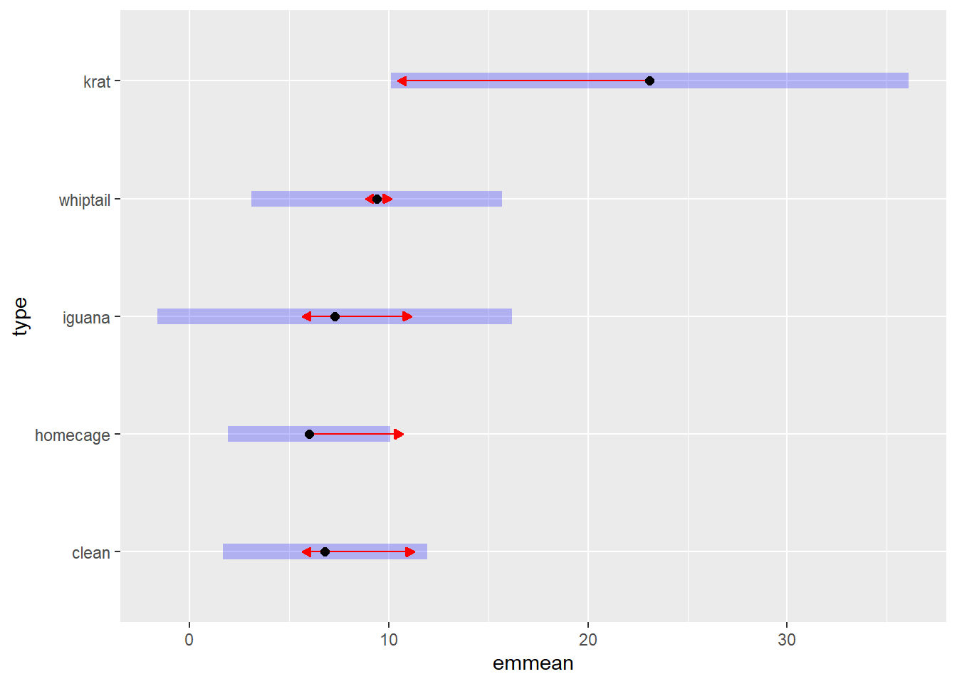
The implementation of a pairwise comparison method that uses a specific error term, in this 1 factor repeated measure design, could easily be done as a dependent samples “t-test”. For example, the comparison of the iguana and whiptail conditions is illustrated. Note that the mean difference is the same as the pairwise comparison just above from emmeans, as are the t value and p values (with the table where adjust was set to “none”). Therefore, this “manual” approach produces the same results as the approach taken above for contrast4 - it is the same hypothesis test (comparing iguana and whiptail conditions). By using the dependent samples t-test for all possible pairs in a post hoc type of approach, the p values could be submitted to the p.adjust function for error rate inflation correction.
t.test(rpt1w.df$iguana, rpt1w.df$whiptail, paired=TRUE)##
## Paired t-test
##
## data: rpt1w.df$iguana and rpt1w.df$whiptail
## t = -1.1485, df = 9, p-value = 0.2804
## alternative hypothesis: true mean difference is not equal to 0
## 95 percent confidence interval:
## -6.236306 2.036306
## sample estimates:
## mean difference
## -2.1Linear Combinations (contrasts) can also be evaluated in the emmeans approach using the contrast function to produce the matrix of coefficients, and the test function to test them. Fortunately, this approach now employs specific error terms that match how we derived them above both from the mlmfit object and where we manually calculated them.
lincombs <- contrast(fit1afex.emm,
               list(type1=c(4, -1,-1,-1,-1),
                    type2=c(0,  3, -1, -1, -1),
                    type3=c(0,  0, -1, -1,  2),
                    type4=c(0,  0, -1,  1,  0)
                    ))
test(lincombs, adjust="none")
## contrast estimate SE df t.ratio p.value
## type1 -18.6 7.44 9 -2.501 0.0338
## type2 -21.8 8.41 9 -2.591 0.0292
## type3 29.5 8.74 9 3.373 0.0082
## type4 2.1 1.83 9 1.148 0.2804A plot and table of confidence intervals for the contrasts can also be obtained, even employing p value adjustments as illustrated here with the bonferroni-sidak adjustment. As was the case when applied to the afex model object, specific error terms are employed. In addition, p value adjustments for the multiple testing problem, are simple to implement with the confint function that produces adjusted confidence intervals for each contrast.
confint(lincombs, adjust="sidak")## contrast estimate SE df lower.CL upper.CL
## type1 -18.6 7.44 9 -41.64 4.44
## type2 -21.8 8.41 9 -47.88 4.28
## type3 29.5 8.74 9 2.40 56.60
## type4 2.1 1.83 9 -3.57 7.77
##
## Confidence level used: 0.95
## Conf-level adjustment: sidak method for 4 estimatesIt is also possible to use the aov_ez flavor of the afex ANOVA functions. This approach also provides specific error terms in the construction of the t-tests for the custom set of contrasts.
First the base/omnibus ANOVA is performed:
contrasts(rpt1.df$type) <- contr.sum
fit2afex.ez <- aov_ez(id="snum",
                      dv="DV",
                      data=rpt1.df,
                      within="type")
summary(fit2afex.ez)
##
## Univariate Type III Repeated-Measures ANOVA Assuming Sphericity
##
## Sum Sq num Df Error SS den Df F value Pr(>F)
## (Intercept) 5533.5 1 3739.7 9 13.3171 0.005324 **
## type 2041.5 4 2077.3 36 8.8447 4.424e-05 ***
## ---
## Signif. codes: 0 '***' 0.001 '**' 0.01 '*' 0.05 '.' 0.1 ' ' 1
##
##
## Mauchly Tests for Sphericity
##
## Test statistic p-value
## type 0.0038542 7.3907e-06
##
##
## Greenhouse-Geisser and Huynh-Feldt Corrections
## for Departure from Sphericity
##
## GG eps Pr(>F[GG])
## type 0.3793 0.005501 **
## ---
## Signif. codes: 0 '***' 0.001 '**' 0.01 '*' 0.05 '.' 0.1 ' ' 1
##
## HF eps Pr(>F[HF])
## type 0.4400688 0.003391046The emmeans contrast approach provides the same specific error terms as when using the aov_car flavor of the afex approach.
fit2.ez.emm <- emmeans(fit2afex.ez, "type", data=rpt1.df)
lincombsez <- contrast(fit2.ez.emm,
               list(type1=c(4, -1,-1,-1,-1),
                    type2=c(0,  3, -1, -1, -1),
                    type3=c(0,  0, -1, -1,  2),
                    type4=c(0,  0, -1,  1,  0)
                    ))
test(lincombsez, adjust="none")
## contrast estimate SE df t.ratio p.value
## type1 -18.6 7.44 9 -2.501 0.0338
## type2 -21.8 8.41 9 -2.591 0.0292
## type3 29.5 8.74 9 3.373 0.0082
## type4 2.1 1.83 9 1.148 0.2804The ability to have emmeans perform the correct contrast tests in this one factor repeated measures ANOVA is welcomed. Its extension to factorial designs is uncertain.
4.5.1 Use of emmeans on aov fit objects.
The emmeans capabilities extend to many model objects beyond afex fits. Unfortunately, when the contrast approach developed above is applied to aov fit objects, the error terms are not specific. But this could be a useful approach when the sphericity assumption is confidently met. In fact, when sphericity is perfect, then all specific error terms will have the exact same numeric value, but df will be smaller than for the omnibus Axs error term - thus less power.
Here, the original aov fit is reproduced and then the emmeans approach for contrasts is applied.
contrasts(rpt1.df$type) <- contr.sum
fit.1 <- aov(DV~type + Error(snum/type), data=rpt1.df)
summary(fit.1)
##
## Error: snum
## Df Sum Sq Mean Sq F value Pr(>F)
## Residuals 9 3740 415.5
##
## Error: snum:type
## Df Sum Sq Mean Sq F value Pr(>F)
## type 4 2042 510.4 8.845 4.42e-05 ***
## Residuals 36 2077 57.7
## ---
## Signif. codes: 0 '***' 0.001 '**' 0.01 '*' 0.05 '.' 0.1 ' ' 1Now the custom contrasts approach; notice the df for the errors are all 36, reflecting use of the omnibus AxS error source rather than specific error terms. The pattern of significant effects is different than with specific error terms. We conclude that the way emmeans and contrast operate on fit objects differs for aov and afex fits. Use of afex fits is preferred.
fit1.aov.emm <- emmeans(fit.1, "type", data=rpt1.df)## Note: re-fitting model with sum-to-zero contrastslincombsaov <- contrast(fit1.aov.emm,
list(type1=c(4, -1,-1,-1,-1),
type2=c(0, 3, -1, -1, -1),
type3=c(0, 0, -1, -1, 2),
type4=c(0, 0, -1, 1, 0)
))
test(lincombsaov, adjust="none")## contrast estimate SE df t.ratio p.value
## type1 -18.6 10.74 36 -1.731 0.0919
## type2 -21.8 8.32 36 -2.620 0.0128
## type3 29.5 5.88 36 5.014 <.0001
## type4 2.1 3.40 36 0.618 0.54044.6 Commentary on Contrast Analysis with the Univariate/Multivariate methods
Even if the first decision is made regarding univariate vs multivariate tests, the user must still decide how to proceed in following up these omnibus tests with pairwise comparisons or analytical/orthogonal contrasts. Unfortunately, the most direct method I have found (“split” argument with an aov object` employs the omnibus error term in creating standard errors or F tests for such comparisons. The only ways to obtain specific error terms are with the manual approaches outlined above or the use of emmeans on an afex model fit. The manual approaches are not terribly burdensome for a simple 1 factor repeated measures design, but will become very much more challenging for larger designs - e.g., two repeated factors or mixed designs with grouping factors and repeated measures factors.
There may be another way of approaching contrasts using the Linear Mixed Models methodology seen in the next chapter. That alternative may provide specific error terms as well.
The conclusion I still hold is that the SPSS MANOVA procedure is efficient and helpful in pursuing these followup contrast types of questions. Its default setting of specific error terms is of considerable value in the MANOVA procedure. It is not clear to me why this has not comprehensively found its way into the R ecosystem such that it is simple to implement. (perhaps there is still something I haven’t yet learned about the suite of R functions employed here, especially perhaps emmeans). In attempts to apply these same strategies to factorial repeated measures designs, the types of error terms used are not so clearly specific. That work is in other tutorial documents.