Chapter 7 Robust and Resampling Methods
A few illustrations of robust methods, permutation testing, and bootstrapping are illustrated here. Some authors treat non-parametric tests as members of the class of robust methods. We have already reviewed that topic in a previous chapter.
7.1 Robust Tests
Wilcox has provided a wealth of robust methods for various inferential tests and designs with the WRS2 package (Mair & Wilcox, 2020). The 1-factor repeated measures design is evaluated with the rmanova function. This function requires the long format data and we will use the initial one first used in this document in chapter 2. The robust method evaluates trimmed means and the “tr” argument specifies the degree of trimming. When tr=0, rmanova replicates the traditional ANOVA and produces the familiar F value from those earlier analyses. I illustrate here with “tr=.2”, but the small number of data points per condition (ten) may mean that this level of trimming is too large. Note that the F statistic from the robust/trimmed approach is smaller than with “tr=0”, but the test is still significant even with reduced/adjusted df.
library(WRS2)
#rmanova(rpt1.df$DV, groups=rpt1.df$type, blocks=rpt1.df$snum, tr=0)
rmanova(rpt1.df$DV, groups=rpt1.df$type, blocks=rpt1.df$snum, tr=.2)
## Call:
## rmanova(y = rpt1.df$DV, groups = rpt1.df$type, blocks = rpt1.df$snum,
## tr = 0.2)
##
## Test statistic: F = 5.6244
## Degrees of freedom 1: 1.32
## Degrees of freedom 2: 6.61
## p-value: 0.04576Also from WRS2, the rmmcp function implements tests of pairwise condition comparisons. Wilcox indicates that the method derives critical p-values using the Rom (1990) method where the alpha level is smaller for comparisons with smaller observed p-values. Rom’s method is a modification of the Hochberg approach to p value adjustment for multiple comparisons. Note that with ten comparisons and the alpha rate correction, power is not high and only one of the comparisons is significant when tr=.2 (none when tr=0). See Wilcox’ writings (Wilcox, 2017) for further explanation. The details are not in the help page for rmmcp. Unlike what Wilcox text says, the current version of rmmcp from WRS2 function does not have an argument to change to the method of Hochberg or other methods of adjusting critical p values.
allpairs1 <- rmmcp(rpt1.df$DV, groups=rpt1.df$type, blocks=rpt1.df$snum, tr=.2)
#str(allpairs1)
allpairs1
## Call:
## rmmcp(y = rpt1.df$DV, groups = rpt1.df$type, blocks = rpt1.df$snum,
## tr = 0.2)
##
## psihat ci.lower ci.upper p.value p.crit sig
## clean vs. homecage 0.83333 -2.81237 4.47903 0.32500 0.02500 FALSE
## clean vs. iguana 0.33333 -4.13565 4.80232 0.73634 0.05000 FALSE
## clean vs. whiptail -1.66667 -8.66274 5.32941 0.30702 0.01690 FALSE
## clean vs. krat -12.33333 -34.36130 9.69464 0.04421 0.00730 FALSE
## homecage vs. iguana 1.16667 -3.49487 5.82820 0.28580 0.01270 FALSE
## homecage vs. whiptail -1.66667 -7.71383 4.38050 0.24540 0.01020 FALSE
## homecage vs. krat -12.50000 -29.68804 4.68804 0.01782 0.00568 FALSE
## iguana vs. whiptail -2.66667 -8.50075 3.16742 0.08093 0.00851 FALSE
## iguana vs. krat -12.00000 -24.04772 0.04772 0.00508 0.00511 TRUE
## whiptail vs. krat -11.16667 -27.77203 5.43870 0.02373 0.00639 FALSEOne could use the p.adjust function to apply other p value adjustment methods. First, we can extract the list of ten p values from the “allpairs1” object.
pvals1 <- allpairs1$comp[1:10,6]
pvals1
## [1] 0.324998613 0.736344309 0.307018998 0.044212265 0.285798317 0.245404979
## [7] 0.017822300 0.080927194 0.005084467 0.023730192Then we can apply the p.adjust function to that vector. Results not shown to save space.
p.adjust(pvals1, method="none")
p.adjust(pvals1, method="bonferroni")
p.adjust(pvals1, method="holm")
p.adjust(pvals1, method="hoch")
p.adjust(pvals1, method="hommel")
p.adjust(pvals1, method="BH")
p.adjust(pvals1, method="BY")
p.adjust(pvals1, method="fdr")
The raw, unadjusted, p values find four of the ten pairs to differ at the nominal .05 alpha level. When using any of the p.adjust methods, no pairs are found to differ. The Rom method has slightly more power and found that one of the pairs, iguana vs krat, differs.
Looking back at all ten pairs of difference, it is interesting to note that the iguana vs krat comparison is not the pair with the largest mean difference (the psihat value). This seeming discrepancy comes about because each test is done as a paired groups test (dependent samples test) and the standard error of the difference can vary between pairs as well as the mean difference. This assertion can be checked by rerunning the rmmcp function without any trimming and then comparing the results from one pair to a dependent samples t-test for the same pair.
rmmcp(rpt1.df$DV, groups=rpt1.df$type, blocks=rpt1.df$snum, tr=0)## Call:
## rmmcp(y = rpt1.df$DV, groups = rpt1.df$type, blocks = rpt1.df$snum,
## tr = 0)
##
## psihat ci.lower ci.upper p.value p.crit sig
## clean vs. homecage 0.8 -4.14409 5.74409 0.56521 0.01690 FALSE
## clean vs. iguana -0.5 -8.02647 7.02647 0.81187 0.05000 FALSE
## clean vs. whiptail -2.6 -7.40129 2.20129 0.07680 0.00851 FALSE
## clean vs. krat -16.3 -35.29012 2.69012 0.01142 0.00730 FALSE
## homecage vs. iguana -1.3 -12.07890 9.47890 0.66683 0.02500 FALSE
## homecage vs. whiptail -3.4 -9.86598 3.06598 0.08429 0.01020 FALSE
## homecage vs. krat -17.1 -36.06142 1.86142 0.00883 0.00568 FALSE
## iguana vs. whiptail -2.1 -8.84647 4.64647 0.28037 0.01270 FALSE
## iguana vs. krat -15.8 -33.89064 2.29064 0.01045 0.00639 FALSE
## whiptail vs. krat -13.7 -28.39754 0.99754 0.00740 0.00511 FALSEt.test(rpt1w.df$iguana, rpt1w.df$krat, paired=T)##
## Paired t-test
##
## data: rpt1w.df$iguana and rpt1w.df$krat
## t = -3.2225, df = 9, p-value = 0.01045
## alternative hypothesis: true mean difference is not equal to 0
## 95 percent confidence interval:
## -26.891493 -4.708507
## sample estimates:
## mean difference
## -15.87.2 Resampling Methods
Both permutation tests and bootstrapping of repeated measures designs would have to focus on resampling the data points within each case/subject/participant. Resampling of cases as a whole would not make sense since that variation is what is “controlled for” by doing the repeated measures analysis. I have not found many illustrations of these methods for repeated measures designs.
7.2.1 Howell’s permutation approach
David Howell has shared R code for manually performing a permutation test with the 1-factor repeated measures design. I have adapted it here for our five-category design.
https://www.uvm.edu/~statdhtx/StatPages/Randomization%20Tests/RepeatedMeasuresAnovaR.html
The approach finds a way to reshuffle the five DV values for each case, randomly and within each case. The primary output is a frequency histogram of all of the F values produced by this procedure - 1000 of them since I specifed the number of resamplings as that value. Note that our observed F value for the data set is actually larger than any of the 1000 permuted samples and thus the empirical p-value is zero, an outcome that is rather extreme.
The function requires the long-format data frame which is imported here once again and given a different name so as to not confuse it with any of the earlier data frames in this document.
A note of caution about this method: I have carefully examined Howell’s code and found that it does accomplish the permutations as intended. However, for our data set, the empirical distribution of F values has a large and suprising majority of values well less than 1.0. This strikes me as an unexpected outcome. Perhaps the non-sphericity in our data set is contributing to the extreme position of our observed F value (8.847) relative to the empirical sampling distribution based on permutations. This requires more exploration.
data <- read.csv("data/1facrpt_long.csv")
# make sure that the case variable is a factor
data$snum <- factor(data$snum)
# change the order of the factor levels of type
# to match the original order
# and match our prior SPSS work, including setting
# up contrasts
data$type <- ordered(data$type,
                     levels=c("clean","homecage","iguana",
                              "whiptail", "krat"))
# specify sum to zero contrasts for the type factor
options(contrasts=c("contr.sum","contr.poly"))
aovbase <- aov(DV~type + Error(snum/type), data = data)
#str(summary(aovbase))
obtF <- summary(aovbase)$"Error: snum:type"[[1]][[4]][1]
#obtF
par( mfrow = c(2,2))
boxplot(data$DV~data$type)
nreps <- 1000
counter <- 0
Fsamp <- numeric(nreps)
levels <- c(1:5)
permTypes <-NULL
orderedType <- data[order(data$type),]
set.seed(12357)
for (i in 1:nreps) {
for (j in 1:10) {
  permTypes <- c(permTypes, sample(levels,5,replace = FALSE))
  }
orderedType$permTypes <- permTypes
sampAOV <- aov(DV~factor(permTypes)+Error(factor(snum)),
               data = orderedType)
Fsamp[i] <- summary(sampAOV)$"Error: Within"[[1]][[4]][1]
if (Fsamp[i] > obtF) counter = counter + 1
permTypes <- NULL
}

p <- counter/nreps
cat("The probability of sampled F greater than obtained F is = ", p, '\n')
## The probability of sampled F greater than obtained F is = 0hist(Fsamp, breaks = 50, bty = "n")
legend(1,50,bquote(paste(p == .(p))), bty = "n" )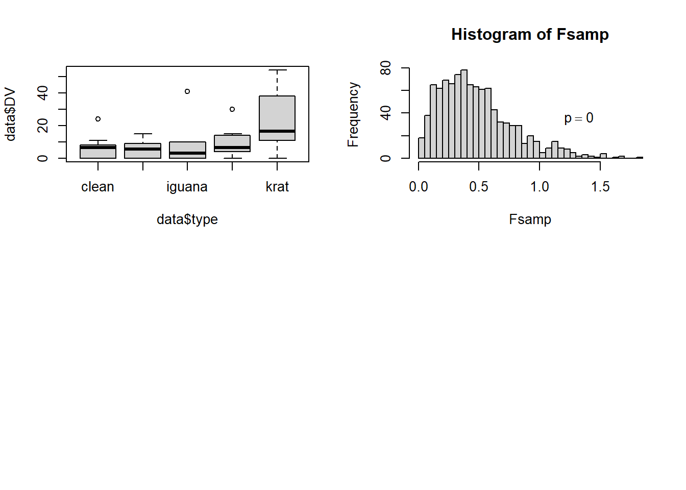
7.3 Bootstrappping
I don’t see much usage of bootstrapping with repeated measures designs, or with more complex factorial designs either. But it can be done although with more complex designs, multiple approaches have to be considered. With our simple 1-factor repeated measures design, the bootstrapping is more straight forward, requiring resampling within each case, across the five conditions. One very easy implementation uses a function provided in the WRS2 package. The rmanovab function implements bootstrapping along with robust estimation using trimmed means. The first illustration here sets the trimming to zero, thus matching the core non-robust approach.
The rmanovab function can use the same long-format data frame that has been the commonly used one in this document. Here, I use the long-format data frame object created just above for the permutation illustration. The function requires two initial arguments specifying the DV and the IV. The number of bootstrap samples is set to 1000 here (probably overkill) and the trimming to zero. The analysis reports the original F value and compares it to the 95th percentile empirical F distribution cutoff. In this illustration our omnibus F exceeds that critical value, so the null is rejected.
Note that in this illustration, trimming is probably not a good idea with only n=10. Doing trimming results in a substantial power loss here. The function help does not make it clear exactly how the bootstrapping is done, and I have some curiosity about whether bootstrapping whole cases has been performed. If that is the case, then it is not clear that it is the best approach. It requires a bit more exploration of Wilcox’ algorithms before I can be fully confident in what the results mean.
library(WRS2)
set.seed(12345)
rmanovab(data$DV, data$type, data$snum, nboot = 1000, tr=0)
## Call:
## rmanovab(y = data$DV, groups = data$type, blocks = data$snum,
## tr = 0, nboot = 1000)
##
## Test statistic: 8.8447
## Critical value: 6.9944
## Significant: TRUEThe pairdepb function is another WRS2 function that does bootstrapping. It produces pairwise comparison tests for all possible pairs. From the function help, it is not clear exactly how the bootstrapping is done and it is surprising that all of the CV are identical and none significant. I need to work through Wilcox’ textbook a bit more on this function before I can recommend it.
## post hoc
set.seed(12354)
pairdepb(data$DV, data$type, data$snum, nboot = 1000, tr=0)
## Call:
## pairdepb(y = data$DV, groups = data$type, blocks = data$snum,
## tr = 0, nboot = 1000)
##
## psihat ci.lower ci.upper test crit sig
## clean vs. homecage 0.8 -6.05004 7.65004 0.45083 6.17647 FALSE
## clean vs. iguana -0.5 -11.20390 10.20390 1.05789 6.17647 FALSE
## clean vs. whiptail -2.6 -16.06131 10.86131 -1.14708 6.17647 FALSE
## clean vs. krat -16.3 -55.36506 22.76506 -2.23985 6.17647 FALSE
## homecage vs. iguana -1.3 -11.53631 8.93631 0.80452 6.17647 FALSE
## homecage vs. whiptail -3.4 -14.69917 7.89917 -1.63989 6.17647 FALSE
## homecage vs. krat -17.1 -54.42551 20.22551 -2.42698 6.17647 FALSE
## iguana vs. whiptail -2.1 -12.16089 7.96089 -2.66027 6.17647 FALSE
## iguana vs. krat -15.8 -51.53824 19.93824 -2.76520 6.17647 FALSE
## whiptail vs. krat -13.7 -43.26975 15.86975 -2.43691 6.17647 FALSE