Chapter 3 Traditional Approaches to One Factor Repeated Measures Designs
The primary goal of this chapter is the elaboration of the traditional “Univariate” approach to the 1-factor Repeated Measures design, evaluation of it’s sphericity assumption. These methods have been the topic of considerable discussion in light of the development of alternatives such as linear mixed effects modeling. Extreme perspectives even argue that the SS partitioning approach of the traditional method is “dead” (McCulloch, 2005). We emphasize that well executed traditional methods, especially those centered on contrast based hypothesis testing, are sound. Later sections in this and other chapters delve into alternative methods. A secondary goal of the chapter is provision of code to implement the multivariate approach to evaluation of the omnibus null hypothesis that all condition means are equal. The multivariate approach is not burdened with the sphericity assumption that has brought the univariate approach under strong criticism. The discussion of which of these to use had been centered around relative power given varying sample sizes and degree of non-sphericity. That conversation has largely been replaced by strong recommendations to use the linear mixed models approach that is outlined in a later chapter. An additional major goal of this document is to explore methods for examining analytical/orthogonal contrasts and pairwise comparison post hoc tests and the stage will be set to produce those analyses in the next chapter.
3.1 The traditional “univariate” GLM approach to the repeated measures problem and the Multivariate approach
The initial sections here, on the univariate approach, emphasize the implementation of the repeated measures design as the theoretical sibling of randomized block designs. It approaches the question in the style of the long litany of experimental design textbooks such as those by Winer, Kirk, Myers, Keppel, and Hays, as well as the current comprehensive textbook by Maxwell, Delaney and Kelley (Hays, 1994; Howell, 2013; Keppel & Wickens, 2004; Kirk, 2013; Myers, Well, & Lorch, 2010; Winer, Brown, & Michels, 1991). In this variance partitioning approach, three sources of variance are identified, owing to the factorial arrangement of the two factors (IV and “subjects/case”:
- “treatment”, the repeated measures factor, called “factor A” in the standard textbook approach.
- “subject” or case (the “blocking” factor)
- The Axs interaction term which will serve as the error term for factor A in this approach.
The theory of the F test from the traditional/univariate approach to omnibus F test for this this one factor repeated measures design is summarized in this table:
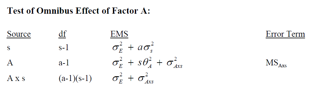
The Axs interaction is usually listed in software output from R as a “residual”. It’s characterization here as an interaction stems from the perspective that a 1 factor repeated measures design is a special case of a randomized block design where the treatment and subject factors are marginal effects (main effects) and the interaction term is possible because each subject is tested under all treatment conditions. In many repeated measures studies, the repeated factor (IV) is characterized simply as a time factor where the same DV is measured at varying time points. In our first example data set, outlined in the previous chapter, the IV was actually a collection of five treatment conditions and each participant was measured under each condition.
The multivariate evaluation approaches the test of the omnibus null hypothesis in a different way, and it is also illustrated in two of the following sections.
The major challenge in replicating the information set that we learned to derive from the SPSS MANOVA or GLM procedure is that there is not simply one function or a small set of functions that can give us everything. That list includes:
In this chapter,
- The omnibus F test of the repeated factor - in some software, this is called the “averaged F test”
- Evaluation of the sphericity assumption
- GG and HF correction factors and adjusted p values
- Implementation the multivariate approach to evaluation of the omnibus null hypothesis
In later chapters we will attempt to add:
- Easy implementation of orthogonal/analytical contrasts
- Error terms specific to the contrasts
- Post hoc evaluation of pairwise comparisons among levels
We will piece these analyses together with several different approaches, and will find that finding correct error terms for contrasts (specific error terms that permit avoidance of the sphericity assumption) is not easily accomplished.
The multiple different ways of accomplishing the omnibus ANOVA found in this chapter can be a bit bewildering. The first method uses the standard/basic approach that employs base system functions. The most efficient approach is probably Method V, using the afex package. The other methods provide alternative strategies that can be helpful in some situations.
3.1.1 Method I: Use of the aov function
Structuring the data set in the “long” format as was done in Chapter 2 permits the standard aov function to partition the variation into the two marginal (main) effects and the interaction term. This requires only a slight change in the code structure compared to the use of aov in “between-subjects” designs. The “Error” argument tells aov that the subject factor is repeated across levels of type. The notation appears to be similar to what we have learned as “nesting”. However, subject is not nested within type as the code might imply with the use of the forward slash, even though some in the R world speak of it that way. It is better to read the notation as implying that all levels of type are found under each subject. It strikes me as an unwieldy way of specifying that the Axs interaction term is the Error term to test the main effect of type. But the whole perspective regarding 1-factor repeated measures designs in R is not conceptually aligned with the randomized block idea - I would wager that most users and many programmers are not aware of the analogy.
It is important to understand that use of the aov function this way has a requirement that the “case” variable (snum here) is a factor. We already specified that factor characteristic in the earlier chapter where the primary data set was imported in chapter 2.
In addition, leaving the contrast set for the “type” factor at the default indicator/dummy coding is not a good idea for repeated measures designs. contr.sum produces deviation/effect coding and either that or orthgonal contrast coding should be employed for repeated measures analyses with the aov and other R methods.
Finally, we need to use the summary function on the aov object, instead of the anova function, in order to produce the traditional SS/df/MS/F/pvalue ANOVA table.
# perform the 1-factor repeated measures anova
# the notation for specification of the error is not intrinsically
# obvious.  some reading in R and S model specification is required.
# always best to use "sum to zero" contrasts for ANOVA
contrasts(rpt1.df$type) <- contr.sum
fit.1 <- aov(DV~type + Error(snum/type), data=rpt1.df)
summary(fit.1)
##
## Error: snum
## Df Sum Sq Mean Sq F value Pr(>F)
## Residuals 9 3740 415.5
##
## Error: snum:type
## Df Sum Sq Mean Sq F value Pr(>F)
## type 4 2042 510.4 8.845 4.42e-05 ***
## Residuals 36 2077 57.7
## ---
## Signif. codes: 0 '***' 0.001 '**' 0.01 '*' 0.05 '.' 0.1 ' ' 1Checking the df for the terms summarized is a doublecheck. We can verify the parallel to the two main effects and the interaction term of the randomized blocks perspective is correct. N was ten, so 9 df for the main effect of snum is correct. Note that summary labels this term “Residuals”. The “type” IV had five levels, so we expected the 4 df for that main effect. And the Axs interaction term should, and does have 9x4=36 df; the interaction term is specified with the “snum:type” notation standard for interactions in aov objects. Once again, summary on this aov object labels this term “Residuals”, a duplicative use of the label but we recognize its Axs identity by understanding the origina of the 36 df. The F and p values match our work with SPSS for this same data set.
One way to quickly obtain additional information is with use of the model.tables function. I obtained the five condition means and the set of deviation effects for each level of type (deviation effects as would be found using effect coding)
#report the means of each level
print(model.tables(fit.1,"means"),digits=3)
## Tables of means
## Grand mean
##
## 10.52
##
## type
## type
## clean homecage iguana whiptail krat
## 6.8 6.0 7.3 9.4 23.1# report deviation effects for each level
print(model.tables(fit.1,"effects", n=TRUE),digits=3) ## Tables of effects
##
## type
## type
## clean homecage iguana whiptail krat
## -3.72 -4.52 -3.22 -1.12 12.58We can evaluate the normality assumption for the residuals with a qqplot. Finding those residuals requires looking at the structure of the fit.1 object and locating the residuals for the Axs interaction. It is in the third section of the list of three components in the fit object (called snum:type here if the `str(fit.1) function is executed). One major outlier is present and there is a hint of positive skew to the distribution but on balance, most of the data points seem to indicate a reasonable fit to the normality assumption. Note that there are only 40 residuals here, but there are 50 data points. The discrepancy is that the original five variables are transformed to contrast vectors and only four vectors are needed for the five-level factor. Thus four new transformed variables and n=10 yields 40 residuals.
#str(fit.1)
qqPlot(resid(fit.1[[3]]),id=FALSE)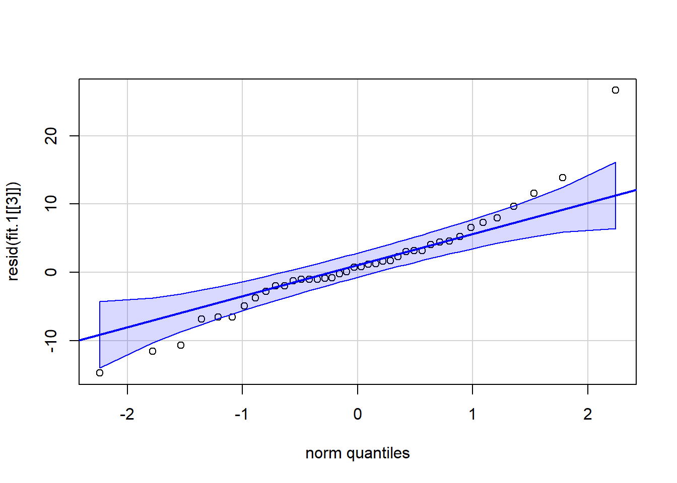
hist(fit.1[[3]]$residuals)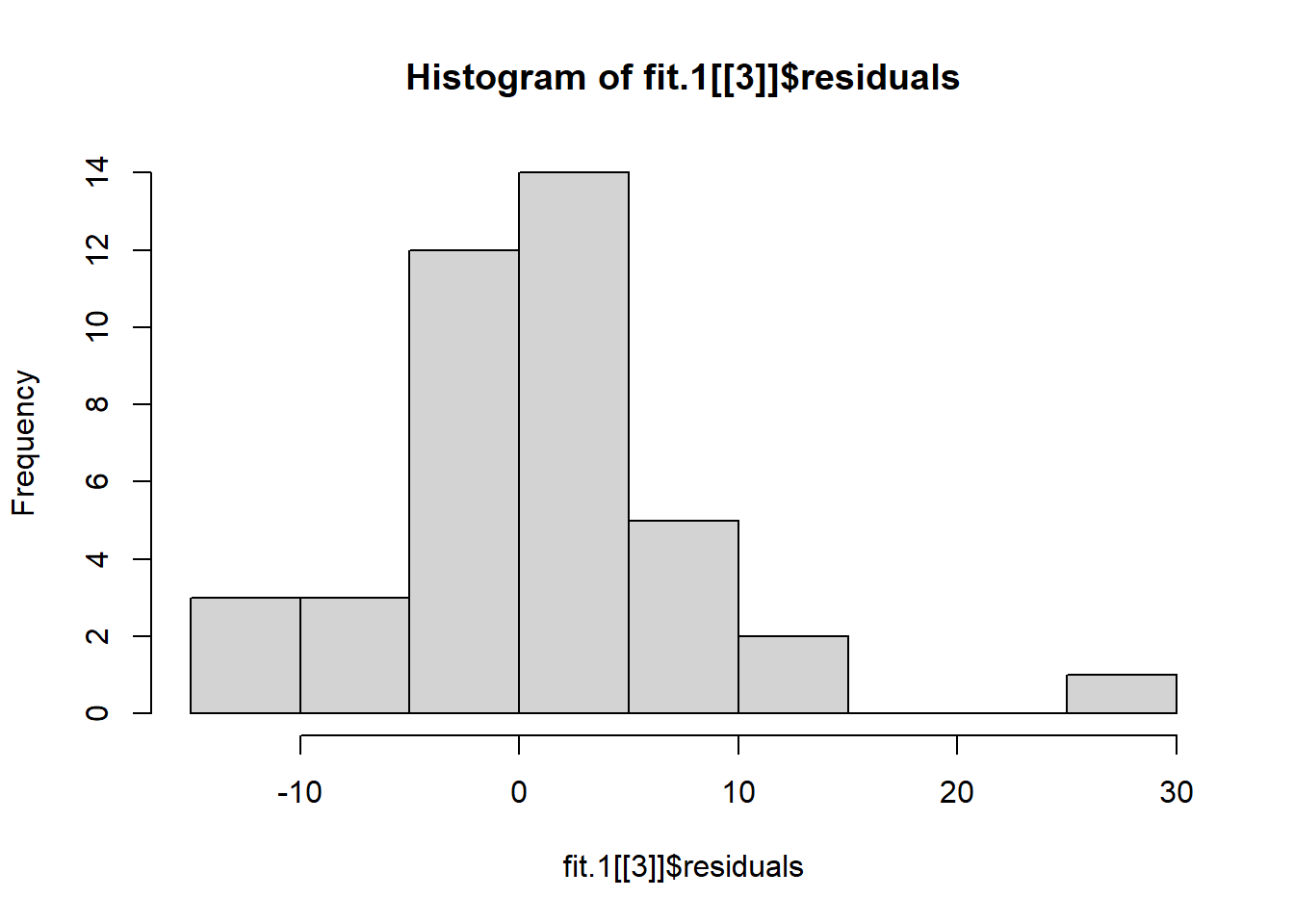
3.1.2 Method II, a multivariate linear model
Method II uses the multivariate linear model. It implements both the multivariate test of the omnibus null hypothesis as well as the averaged F test approach with GG and HF corrections. It also permits the user to obtain the Mauchly Sphericity test and GG/HF corrections.
This approach requires the data frame to be “wide”, AND, only contain the variables that are the levels of the repeated factor. No additional variables such as a subject code can exist in the matrix of variables that is created from the data frame.
This appproach is modeled after an article by Dalgaard:
http://www.r-project.org/doc/Rnews/Rnews_2007-2.pdf
This approach requires the “wide” version of the data file, and that file is available as the .csv file loaded here. The functions to be used require that the data be in matrix form, not as a data frame. So, that conversion is also accomplished here, following data import.
# read data file
rpt1w.df <- read.table("data/1facrpt_wide1.csv",header=T,sep=",")
# change the data from a data frame to a matrix,
# leaving out the snum variable.
# this method requires that the matrix contains
# only the data values
rpt1w.mat <- as.matrix(rpt1w.df)[,2:6]
# view the data
rpt1w.mat
## clean homecage iguana whiptail krat
## [1,] 24 15 41 30 50
## [2,] 6 6 0 6 13
## [3,] 4 0 5 4 9
## [4,] 11 9 10 14 18
## [5,] 0 0 0 0 0
## [6,] 8 15 10 15 38
## [7,] 8 5 2 6 15
## [8,] 0 0 0 11 54
## [9,] 0 3 1 1 11
## [10,] 7 7 4 7 23The multivariate linear model is based on use of the standard lm function. The model specification argument uses the “~1” syntax to indicate that all variable in the matrix are to be included. Then the estVar function can be used to visualize the variance-covariance matrix of the five variables.
# first fit the five variate model to get the var/cov matrix
mlmfit.1 <- lm(rpt1w.mat~1)
estVar(mlmfit.1)
## clean homecage iguana whiptail krat
## clean 51.51111 32.88889 82.40000 55.97778 58.46667
## homecage 32.88889 32.22222 50.88889 39.44444 49.22222
## iguana 82.40000 50.88889 154.90000 99.42222 122.41111
## whiptail 55.97778 39.44444 99.42222 77.37778 124.51111
## krat 58.46667 49.22222 122.41111 124.51111 330.32222# doublecheck with the `cov` function
#cov(rpt1w.mat)Next, an intercept only model is fit by removing the variates from the full model using the update function.
# now fit an intercept only model and use the
# anova function in the next section to compare models,
mlmfit.0 <- update(mlmfit.1, ~0)
#estVar(mlmfit.0)
A test based on multivariate normal theory evaluates an hypothesis that all variates (repeated measures levels) have equal means is possible with this syntax. A model comparison approach is used by passing the two models created above to the anova function. The Pillai test statistic, approximate F value, df and p value match what we produced in SPSS. This test does not have the sphericity assumption. The multivariate test is evaluated as the degree of improvement in fiit (or reduction in residuals) in the full model (mlmfit.1) relative to the intercept-only model (mlmfit.0).
anova(mlmfit.1, mlmfit.0, X=~1)## Analysis of Variance Table
##
## Model 1: rpt1w.mat ~ 1
## Model 2: rpt1w.mat ~ 1 - 1
##
## Contrasts orthogonal to
## ~1
##
## Res.Df Df Gen.var. Pillai approx F num Df den Df Pr(>F)
## 1 9 9.6149
## 2 10 1 11.2467 0.64954 2.7801 4 6 0.1269The Mauchly test can be performed on the mlmfit.1 object. The W test statistic and p value match our SPSS MANOVA results.
mauchly.test(mlmfit.1, X=~1)##
## Mauchly's test of sphericity
## Contrasts orthogonal to
## ~1
##
##
## data: SSD matrix from lm(formula = rpt1w.mat ~ 1)
## W = 0.0038542, p-value = 7.391e-06The univariate averaged F test can also be produced by adding the “test” argument. This produces the same F value as we derived with the standard ANOVA approach in SPSS MANOVA, the approach that assumes sphericity. Note that the GG and HF epsilons are produced and that the adjustment produces the same p values as we obtained in MANOVA.
anova(mlmfit.1, mlmfit.0, X=~1, test="Spherical")## Analysis of Variance Table
##
## Model 1: rpt1w.mat ~ 1
## Model 2: rpt1w.mat ~ 1 - 1
##
## Contrasts orthogonal to
## ~1
##
## Greenhouse-Geisser epsilon: 0.3793
## Huynh-Feldt epsilon: 0.4401
##
## Res.Df Df Gen.var. F num Df den Df Pr(>F) G-G Pr H-F Pr
## 1 9 9.6149
## 2 10 1 11.2467 8.8447 4 36 4.4236e-05 0.0055009 0.003391While Method II gives the multivariate test and provides another way to obtain the traditional univariate F test along with GG and HF corrections (as well as the Mauchly test) it has a downside. The model specification formulae are difficult arguments for the relative novice at R programming, especially the ~1 and ~0 types of structures. There is also not a simple way to extract tests of contrasts with this approach, that I have found. Method III uses a similar underlying logic, but is simpler to implement.
3.1.3 Method III, also a Multivariate Linear Model but using Anova from car
Method III is similar to Method II, but uses an Anova approach in John Fox’s car package that permits the Mauchly test and the GG and HF corrections as well as permitting Type III sums of squares (which lm and anova does not. However, Type III SS is not relevant here - since there are no missing data points, the data set is balanced. But this approach can be useful for advanced designs that contain both repeated measures factors and between-groups factors as well as unequal N.
# use the same "wide" data frame as from Method II
# change the data from a data frame to a matrix
# and leave out the snum variable
# this method requires that the matrix only contains the data values
rpt1w.mat <- as.matrix(rpt1w.df[,-1])
# view the data
rpt1w.mat
## clean homecage iguana whiptail krat
## [1,] 24 15 41 30 50
## [2,] 6 6 0 6 13
## [3,] 4 0 5 4 9
## [4,] 11 9 10 14 18
## [5,] 0 0 0 0 0
## [6,] 8 15 10 15 38
## [7,] 8 5 2 6 15
## [8,] 0 0 0 11 54
## [9,] 0 3 1 1 11
## [10,] 7 7 4 7 23# start by defining the multivariate linear model
# this code returns the level means.
mlmfit.2 <- lm(rpt1w.mat ~1)
mlmfit.2##
## Call:
## lm(formula = rpt1w.mat ~ 1)
##
## Coefficients:
## clean homecage iguana whiptail krat
## (Intercept) 6.8 6.0 7.3 9.4 23.1The completion of the analysis requires the creation of the repeated measures factor. The data set, in the wide format, is simply a collection of five variables. The “type” variable used in Method I does not exist. So we need to create an object that is that five-level factor. The factor is also “ordered” to keep the levels in the same order as was done above for graphing purposes, but also to have the upcoming contrast analysis match what we did in SPSS MANOVA. The creation of this “stimulus” factor (really the same thing as “type” in the long format data set) is analogous to using the “wsfactors” subcommand in SPSS MANOVA and GLM. My choice of the word “stimulus” is shorthand for “stimulus type” and this reinforces the identity to the “type” variable as used in Method I.
# now define a variable that gives the design of the study,
# the levels of the repeated factor, and order them the
# same way that we did in the original SPSS analyses
stimulus <- factor(c("clean", "homecage", "iguana" ,
                     "whiptail", "krat"))
stimulus  <- ordered(stimulus,
                     levels=c("clean","homecage","iguana",
                              "whiptail", "krat"))
stimulus
## [1] clean homecage iguana whiptail krat
## Levels: clean < homecage < iguana < whiptail < kratThe implementation of the analysis with this approach focuses on use of the Anova function from the car package. Two crucial arguments are required to specify the repeated measures nature of the analysis of the design. These are the “idata” and “idesign” arguments. Anova uses the multivariate object defined above and then applies the idesign specification. Applying summary to that Anova object produces the multivariate and univariate tests of the omnibus hypothesis. It also provides the Mauchly test of sphericity, the GG and HF epsilons, and corrected univariate test p-values, all matching the Method II and SPSS results. The terms “idesign”, “idata”, and “icontrasts” derive from the phrase “Intra-subject” which implies repeated measures.
When using the idesign argument, Anova transforms the levels of the repeated measures factors into orthogonal contrasts. Look carefully at the product of the summary function here and see if you can guess what this default set of contrasts is. Hint:
it is the default because the most common type of repeated measure factor is a collection of measurements at various time points, and is thus a quantitative IV.
There may be something that I am missing about using this method, but I can’t sort out a direct way of testing the contrasts. This is in spite of the fact that their SS are reported. We will return to this with a manual method in a later section of the next chapter.
#require(car)
mlmfit2.anova <- Anova(mlmfit.2,
                       idata=data.frame(stimulus),
                       idesign=~stimulus, type="III")
# with the summary function, when multivariate=TRUE,
# and univariate=TRUE,
# both multivariate and averaged F tests of the
# repeated effect are printed.
summary(mlmfit2.anova, multivariate=T, univariate=T)
##
## Type III Repeated Measures MANOVA Tests:
##
## ------------------------------------------
##
## Term: (Intercept)
##
## Response transformation matrix:
## (Intercept)
## clean 1
## homecage 1
## iguana 1
## whiptail 1
## krat 1
##
## Sum of squares and products for the hypothesis:
## (Intercept)
## (Intercept) 27667.6
##
## Multivariate Tests: (Intercept)
## Df test stat approx F num Df den Df Pr(>F)
## Pillai 1 0.5967217 13.3171 1 9 0.0053237 **
## Wilks 1 0.4032783 13.3171 1 9 0.0053237 **
## Hotelling-Lawley 1 1.4796774 13.3171 1 9 0.0053237 **
## Roy 1 1.4796774 13.3171 1 9 0.0053237 **
## ---
## Signif. codes: 0 '***' 0.001 '**' 0.01 '*' 0.05 '.' 0.1 ' ' 1
##
## ------------------------------------------
##
## Term: stimulus
##
## Response transformation matrix:
## stimulus.L stimulus.Q stimulus.C stimulus^4
## clean -0.6324555 0.5345225 -3.162278e-01 0.1195229
## homecage -0.3162278 -0.2672612 6.324555e-01 -0.4780914
## iguana 0.0000000 -0.5345225 -4.095972e-16 0.7171372
## whiptail 0.3162278 -0.2672612 -6.324555e-01 -0.4780914
## krat 0.6324555 0.5345225 3.162278e-01 0.1195229
##
## Sum of squares and products for the hypothesis:
## stimulus.L stimulus.Q stimulus.C stimulus^4
## stimulus.L 1296.0000 906.6815 342.00000 164.64132
## stimulus.Q 906.6815 634.3143 239.26317 115.18306
## stimulus.C 342.0000 239.2632 90.25000 43.44702
## stimulus^4 164.6413 115.1831 43.44702 20.91571
##
## Multivariate Tests: stimulus
## Df test stat approx F num Df den Df Pr(>F)
## Pillai 1 0.6495405 2.780095 4 6 0.12692
## Wilks 1 0.3504595 2.780095 4 6 0.12692
## Hotelling-Lawley 1 1.8533965 2.780095 4 6 0.12692
## Roy 1 1.8533965 2.780095 4 6 0.12692
##
## Univariate Type III Repeated-Measures ANOVA Assuming Sphericity
##
## Sum Sq num Df Error SS den Df F value Pr(>F)
## (Intercept) 5533.5 1 3739.7 9 13.3171 0.005324 **
## stimulus 2041.5 4 2077.3 36 8.8447 4.424e-05 ***
## ---
## Signif. codes: 0 '***' 0.001 '**' 0.01 '*' 0.05 '.' 0.1 ' ' 1
##
##
## Mauchly Tests for Sphericity
##
## Test statistic p-value
## stimulus 0.0038542 7.3907e-06
##
##
## Greenhouse-Geisser and Huynh-Feldt Corrections
## for Departure from Sphericity
##
## GG eps Pr(>F[GG])
## stimulus 0.3793 0.005501 **
## ---
## Signif. codes: 0 '***' 0.001 '**' 0.01 '*' 0.05 '.' 0.1 ' ' 1
##
## HF eps Pr(>F[HF])
## stimulus 0.4400688 0.003391046The multivariate tests match what was seen in Method II above, as does the Univariate F test which also matches the F test seen with Method I. The “Sum of squares and products for the hypothesis” matrix provides a starting point for evaluating contrasts and this will be developed in the next chapter.
3.1.4 Method IV: Implement the univariate analysis with ezanova from the ez package
The ezanova function is a wrapper for the aov function and may be simpler to use than the aov function for some designs. It has the added value of performing the Mauchly sphericity test and providing GG and HF epsilons and corrected p values as well as an effect size indicator. The structure of the code requires an argument for the data frame (needs the long format data frame), the dependent variable, the ID factor for the case variable (subject, or snum in our data set), and the repeated measures factor (the within argument).
This might be the simplest of all approaches to obtain the omnibus F test plus the sphericity test and associated corrections. The main arguments that create the repeated measures analysis are “dv” which is the dependent variable name, “wid” which is the subject variable ID code (and the period is a odd but necessary part of the code) and “within” which is the repeated measure IV.
#library(ez)
fit1.ez <- ezANOVA(data=rpt1.df, detailed=T, return_aov=T,
                   dv=DV,
                   wid=.(snum),
                   within=.(type))
fit1.ez
## $ANOVA
## Effect DFn DFd SSn SSd F p p<.05 ges
## 1 (Intercept) 1 9 5533.52 3739.68 13.317097 5.323652e-03 * 0.4875125
## 2 type 4 36 2041.48 2077.32 8.844723 4.423582e-05 * 0.2597805
##
## $`Mauchly's Test for Sphericity`
## Effect W p p<.05
## 2 type 0.003854226 7.390741e-06 *
##
## $`Sphericity Corrections`
## Effect GGe p[GG] p[GG]<.05 HFe p[HF] p[HF]<.05
## 2 type 0.3792955 0.005500897 * 0.4400688 0.003391046 *
##
## $aov
##
## Call:
## aov(formula = formula(aov_formula), data = data)
##
## Grand Mean: 10.52
##
## Stratum 1: snum
##
## Terms:
## Residuals
## Sum of Squares 3739.68
## Deg. of Freedom 9
##
## Residual standard error: 20.38431
##
## Stratum 2: snum:type
##
## Terms:
## type Residuals
## Sum of Squares 2041.48 2077.32
## Deg. of Freedom 4 36
##
## Residual standard error: 7.596271
## Estimated effects may be unbalanced3.1.5 Method V: Implement the univariate analysis with the afex package
The afex package permits specification of repeated measures models using styles from ez, aov, lm, car::Anova and other modeling functions. Here, the code reflects the basic aov syntax for the model specification and uses Anova from car for calculations.
This initial approach requests the base univariate/averaged F approach, first setting the contrasts to the “sum to zero” contrast set that should be done for ANOVA designs, especially repeated measures - orthogonal contrasts are also “sum to zero” contrasts and will be examined in a later chapter. Here, the contr.sum specification sets the contrasts to “effect” coding.
contrasts(rpt1.df$type) <- contr.sum
fit1.afex <- aov_car(DV~type + Error(snum/type), data=rpt1.df)
summary(fit1.afex)
##
## Univariate Type III Repeated-Measures ANOVA Assuming Sphericity
##
## Sum Sq num Df Error SS den Df F value Pr(>F)
## (Intercept) 5533.5 1 3739.7 9 13.3171 0.005324 **
## type 2041.5 4 2077.3 36 8.8447 4.424e-05 ***
## ---
## Signif. codes: 0 '***' 0.001 '**' 0.01 '*' 0.05 '.' 0.1 ' ' 1
##
##
## Mauchly Tests for Sphericity
##
## Test statistic p-value
## type 0.0038542 7.3907e-06
##
##
## Greenhouse-Geisser and Huynh-Feldt Corrections
## for Departure from Sphericity
##
## GG eps Pr(>F[GG])
## type 0.3793 0.005501 **
## ---
## Signif. codes: 0 '***' 0.001 '**' 0.01 '*' 0.05 '.' 0.1 ' ' 1
##
## HF eps Pr(>F[HF])
## type 0.4400688 0.003391046The inital approach does not produce an effect size estimate. One way to obtain the “generalized effect size” statistic is to simply ask to see the afex fit object, but as a stand alone method this may not be desireable since it only reports the GG corrected p value.
fit1.afex## Anova Table (Type 3 tests)
##
## Response: DV
## Effect df MSE F ges p.value
## 1 type 1.52, 13.65 152.13 8.84 ** .260 .006
## ---
## Signif. codes: 0 '***' 0.001 '**' 0.01 '*' 0.05 '+' 0.1 ' ' 1
##
## Sphericity correction method: GGA more full way of taking control is to use the “anova_table” argument in the original aov_car specification. The correction argument in the “anova_table” list permits “none”, “GG” or “HF” for sphericity corrections. Simply asking for a printout of the fit2.afex object also yields the corrected p value (or uncorrected as is requested here) and an effect size statistic. The options for the “es” specification are “pes” for partial eta squared, and “ges” for the generalized effect size. See the help pages for the afex functions for references regarding the generalized effect size statistic if that has not yet been covered in class.
# make sure "sum to zero" contrasts are specified - done above
fit2.afex <- aov_car(DV~type + Error(snum/type), data=rpt1.df,
                     anova_table = list(correction = "none", es="pes"))
fit2.afex
## Anova Table (Type 3 tests)
##
## Response: DV
## Effect df MSE F pes p.value
## 1 type 4, 36 57.70 8.84 *** .496 <.001
## ---
## Signif. codes: 0 '***' 0.001 '**' 0.01 '*' 0.05 '+' 0.1 ' ' 1An example of using one of the correction methods and a choice of the “ges” effect size is next:
# make sure "sum to zero" contrasts are specified - done above
fit3.afex <- aov_car(DV~type + Error(snum/type), data=rpt1.df,
                     anova_table = list(correction = "HF", es="ges"))
fit3.afex
## Anova Table (Type 3 tests)
##
## Response: DV
## Effect df MSE F ges p.value
## 1 type 1.76, 15.84 131.12 8.84 ** .260 .003
## ---
## Signif. codes: 0 '***' 0.001 '**' 0.01 '*' 0.05 '+' 0.1 ' ' 1
##
## Sphericity correction method: HFNeither of these previous two code chunks provide the sphericity test. That can be done by applying the summary function to the aov_car objects. For example…..:
summary(fit3.afex)##
## Univariate Type III Repeated-Measures ANOVA Assuming Sphericity
##
## Sum Sq num Df Error SS den Df F value Pr(>F)
## (Intercept) 5533.5 1 3739.7 9 13.3171 0.005324 **
## type 2041.5 4 2077.3 36 8.8447 4.424e-05 ***
## ---
## Signif. codes: 0 '***' 0.001 '**' 0.01 '*' 0.05 '.' 0.1 ' ' 1
##
##
## Mauchly Tests for Sphericity
##
## Test statistic p-value
## type 0.0038542 7.3907e-06
##
##
## Greenhouse-Geisser and Huynh-Feldt Corrections
## for Departure from Sphericity
##
## GG eps Pr(>F[GG])
## type 0.3793 0.005501 **
## ---
## Signif. codes: 0 '***' 0.001 '**' 0.01 '*' 0.05 '.' 0.1 ' ' 1
##
## HF eps Pr(>F[HF])
## type 0.4400688 0.003391046Finally, we can examine use of the other afex functions that provide the same general approach, but uses the style of model specification from the ‘ez’ package. First, the “ez” style:
# make sure "sum to zero" contrasts are specified - done above
fit4.afex <- aov_ez(data=rpt1.df, detailed=T, return_aov=T,
                   dv="DV",
                   id="snum",
                   within="type",
                     anova_table = list(correction = "HF", es="ges"))
fit4.afex
## Anova Table (Type 3 tests)
##
## Response: DV
## Effect df MSE F ges p.value
## 1 type 1.76, 15.84 131.12 8.84 ** .260 .003
## ---
## Signif. codes: 0 '***' 0.001 '**' 0.01 '*' 0.05 '+' 0.1 ' ' 1
##
## Sphericity correction method: HFsummary(fit4.afex)##
## Univariate Type III Repeated-Measures ANOVA Assuming Sphericity
##
## Sum Sq num Df Error SS den Df F value Pr(>F)
## (Intercept) 5533.5 1 3739.7 9 13.3171 0.005324 **
## type 2041.5 4 2077.3 36 8.8447 4.424e-05 ***
## ---
## Signif. codes: 0 '***' 0.001 '**' 0.01 '*' 0.05 '.' 0.1 ' ' 1
##
##
## Mauchly Tests for Sphericity
##
## Test statistic p-value
## type 0.0038542 7.3907e-06
##
##
## Greenhouse-Geisser and Huynh-Feldt Corrections
## for Departure from Sphericity
##
## GG eps Pr(>F[GG])
## type 0.3793 0.005501 **
## ---
## Signif. codes: 0 '***' 0.001 '**' 0.01 '*' 0.05 '.' 0.1 ' ' 1
##
## HF eps Pr(>F[HF])
## type 0.4400688 0.003391046And next, the “lme” style:
# make sure "sum to zero" contrasts are specified - done above
fit5.afex <- aov_4(DV ~ type  + (type|snum), data=rpt1.df,
                     anova_table = list(correction = "none", es="ges"))
fit5.afex
## Anova Table (Type 3 tests)
##
## Response: DV
## Effect df MSE F ges p.value
## 1 type 4, 36 57.70 8.84 *** .260 <.001
## ---
## Signif. codes: 0 '***' 0.001 '**' 0.01 '*' 0.05 '+' 0.1 ' ' 1summary(fit5.afex)##
## Univariate Type III Repeated-Measures ANOVA Assuming Sphericity
##
## Sum Sq num Df Error SS den Df F value Pr(>F)
## (Intercept) 5533.5 1 3739.7 9 13.3171 0.005324 **
## type 2041.5 4 2077.3 36 8.8447 4.424e-05 ***
## ---
## Signif. codes: 0 '***' 0.001 '**' 0.01 '*' 0.05 '.' 0.1 ' ' 1
##
##
## Mauchly Tests for Sphericity
##
## Test statistic p-value
## type 0.0038542 7.3907e-06
##
##
## Greenhouse-Geisser and Huynh-Feldt Corrections
## for Departure from Sphericity
##
## GG eps Pr(>F[GG])
## type 0.3793 0.005501 **
## ---
## Signif. codes: 0 '***' 0.001 '**' 0.01 '*' 0.05 '.' 0.1 ' ' 1
##
## HF eps Pr(>F[HF])
## type 0.4400688 0.003391046This implementation with afex is probably the simplest way to accomplish the primary requirements of finding the omnibus F test, evaluating the sphericity assumption, correcting the p value for any sphericity violations, and providing an effect size estimate. The approach taken for fit2.afex, along with use of the summary function on that object strikes me as the most efficient way of doing the traditional omnibus ANOVA. Objects from these afex functions also provide a direct way to interface with the emmeans approach to contrasts and post hoc testing found in a later chapter.
3.2 Commentary on the Univariate/Multivariate methods
The user has two kinds of decisions to make. The first is whether the multivariate GLM approach is desired, or the univariate one (the averaged F test). Method II and Method III produce both types of test and the choice depends, in part on examination of the sphericity assumption. The real question is whether to use the multivariate test or the GG/HF corrected univariate approach. Typically researchers have not frequently used the multivariate approach because of its relative low power for the typical small sample sizes of many repeated measures experiments. A literature on the relative merits of the two approaches can be found in your textbooks and the Dudek stat toolkit bibliography.
Of all the methods, the simplest to implement might be method V, using afex. This provides the sphericity test and GG/HF corrections to the univariate p value for the omnibus test. If the user does not prefer the corrected univariate test in the face of non-sphericity, then Method I, II or Method III can be employed once the sphericity assumption is examined (from Method II or III).