Chapter 5 Linear Mixed Models
As an alternative to the traditional methods found in Chapter 3, this chapter briefly introduces Linear Mixed Effects Modeling. Although at this point in the course we have not covered any of the theory of LMM, we can examine the basics of implementation for this simple one-factor repeated measures design. LMM is a class of techniques that handle nested/hierarchical designs, and longitudinal growth curve modeling of which repeated measures designs can be seen as a subset. This suite of methods is designed to handle random factors such as “subjects” in a repeated measures design. The major advantages of LMM approaches to repeated measures are:
Can handle missing data. The traditional approaches usually employ casewise deletion if any data points are missing for a case.
Can handle repeated factors such as time where not all participants are measured at exactly the same time points or that vary in total number of time points measured.
Can specify alternative covariance strutures to the compound symmetry and sphericity patterns that the traditional methods assume.
Of these, the only one that is important for the one-factor design that is illustrated here is the last point.
The illustrations here use two different packages, nlme and lme4. Detailed training in these methods is advised before routine usage.
5.1 Basic LMM Analysis using lme
Here, I illustrate the lme function from nlme. It requires the same long-format data frame as the aov function we used for the traditional analysis. That data set is imported again here, along with the changes of “snum” to a factor and reordering the “type” variable levels.
# need "long" form of the data set as in Method I of chapter 3
rpt1.df <- read.csv("data/1facrpt_long.csv")
# change the snum variable to a factor variable (was numeric)
rpt1.df$snum <- as.factor(rpt1.df$snum)
rpt1.df$type <- ordered(rpt1.df$type,
                        levels=c("clean","homecage","iguana",
                                 "whiptail", "krat"))
# look at beginning and ending few lines of the  data frame
gt(headTail(rpt1.df))| snum | type | DV |
|---|---|---|
| 1 | clean | 24 |
| 1 | homecage | 15 |
| 1 | iguana | 41 |
| 1 | whiptail | 30 |
| NA | NA | ... |
| 10 | homecage | 7 |
| 10 | iguana | 4 |
| 10 | whiptail | 7 |
| 10 | krat | 23 |
The syntax of the lme function is somewhat similar to the aov/lm syntax. The most important specification is the way that the random factor is specified. The ~1|snum/type specification is not intuitively obvious. Understanding it requires a background in the theory of LMM and a careful reading of the R help page on the function, neither of which will be reviewed here.
Initially, we fit a model that contains all of the specifics required for the overall/omnibus model evaluation. Note that we examine the model with the standard anova and summary functions that we have become familiar with in other ANOVA/regression analyses.
In interpreting this initial output, several things become apparent:
- The
anovaoutput yields the same F and p value as the traditional Univariate approach. This is because the traditional GLM approach can be viewed as a subset of types of LMM analyses and the default covariance structure is the one of compound symmetry, and that would be a problematic assumption here too. summaryproduces information criteria (AIC/BIC) as well as info on the overall intercept (related to the overall mean) and a term that indicates that the intercept is permitted to vary across subjects (related to the Axs interaction).- Information on coefficients reflects the fact that individual contrast vectors were created and by default, they are those of trend analysis. This is because the defaults presume that the repeated measure is a time-related factor and that trend would thus be desireable. Since this is not the case for our illustration the succeeding code chunks changes the contrasts and we re-run the analysis.
#require(nlme)
# first, default, LMM model assumes sphericity and reproduces  the
# omnibus F test produced as the "average F" in the SPSS MANOVA approach
fit1.lme <- lme(DV ~ type, random = ~1|snum/type, data=rpt1.df)
anova(fit1.lme)
## numDF denDF F-value p-value
## (Intercept) 1 36 13.317097 8e-04
## type 4 36 8.844723 <.0001summary(fit1.lme)## Linear mixed-effects model fit by REML
## Data: rpt1.df
## AIC BIC logLik
## 357.0839 371.5372 -170.542
##
## Random effects:
## Formula: ~1 | snum
## (Intercept)
## StdDev: 8.459511
##
## Formula: ~1 | type %in% snum
## (Intercept) Residual
## StdDev: 6.930132 3.110725
##
## Fixed effects: DV ~ type
## Value Std.Error DF t-value p-value
## (Intercept) 10.520000 2.882776 36 3.649260 0.0008
## type.L 11.384200 2.402152 36 4.739167 0.0000
## type.Q 7.964385 2.402152 36 3.315521 0.0021
## type.C 3.004164 2.402152 36 1.250614 0.2191
## type^4 1.446227 2.402152 36 0.602055 0.5509
## Correlation:
## (Intr) type.L type.Q type.C
## type.L 0
## type.Q 0 0
## type.C 0 0 0
## type^4 0 0 0 0
##
## Standardized Within-Group Residuals:
## Min Q1 Med Q3 Max
## -0.756930607 -0.157209242 -0.003407451 0.137647579 1.550657810
##
## Number of Observations: 50
## Number of Groups:
## snum type %in% snum
## 10 50In this next section, we recreate the same set of orthogonal contrasts used for analyses in the traditional approaches found in chapter 3.
# now create contrasts for the type factor
contrasts.type <- matrix(c(4, -1, -1, -1, -1,
                           0,  3, -1, -1, -1,
                           0,  0, -1, -1,  2,
                           0,  0, -1,  1,  0),
                         ncol=4)
contrasts(rpt1.df$type) <- contrasts.type
contrasts(rpt1.df$type)
## [,1] [,2] [,3] [,4]
## clean 4 0 0 0
## homecage -1 3 0 0
## iguana -1 -1 -1 -1
## whiptail -1 -1 -1 1
## krat -1 -1 2 0Fitting the model again now employs those orthogonal contrasts. Note that the t values in the summary table below for these contrasts are not the same as those we found in chapter 4 using the “manual” method or from our SPSS work. They do match the t and p values found in using emmeans in chapter 4. The “estimates” shown in the table are correct, reflecting the fact that the contrast coefficients have been orthonormalized. For example, multiple the first “estimate” (for type1) by 20 (the sum of the squared coefficients) and the value is -18.6, the mean of the manually created vector for contrast 1 that was done in chapter 3. The std errors and the df for the error reveal why there is a mismatch. In this analysis that is essentially a reproduction of the GLM approach, the 36 df for the error reveals the fact that errors are not specific to the contrast - the omnibus Axs MS is used in the error. This recreates the same problem with the sphericity assumption that the GLM approach has if the omnibus Axs error term is used for contrasts.
fit2.lme <- lme(DV ~ type, random = ~1|snum/type,   data=rpt1.df)
anova(fit2.lme)
## numDF denDF F-value p-value
## (Intercept) 1 36 13.317097 8e-04
## type 4 36 8.844723 <.0001summary(fit2.lme)## Linear mixed-effects model fit by REML
## Data: rpt1.df
## AIC BIC logLik
## 365.0495 379.5028 -174.5247
##
## Random effects:
## Formula: ~1 | snum
## (Intercept)
## StdDev: 8.459511
##
## Formula: ~1 | type %in% snum
## (Intercept) Residual
## StdDev: 6.930132 3.110725
##
## Fixed effects: DV ~ type
## Value Std.Error DF t-value p-value
## (Intercept) 10.520000 2.8827764 36 3.649260 0.0008
## type1 -0.930000 0.5371375 36 -1.731400 0.0919
## type2 -1.816667 0.6934415 36 -2.619784 0.0128
## type3 4.916667 0.9806744 36 5.013557 0.0000
## type4 1.050000 1.6985778 36 0.618164 0.5404
## Correlation:
## (Intr) type1 type2 type3
## type1 0
## type2 0 0
## type3 0 0 0
## type4 0 0 0 0
##
## Standardized Within-Group Residuals:
## Min Q1 Med Q3 Max
## -0.756930607 -0.157209242 -0.003407451 0.137647579 1.550657810
##
## Number of Observations: 50
## Number of Groups:
## snum type %in% snum
## 10 50The phia package has a function called testInteractions that can work on a lme model object. This function is built to handle factorial designs, and thus the name testInteractions. But it can handle main effect contrasts which is what we have in this one-factor design (that can be conceived as a two factor randomized blocks design). In testing it for the first contrast, the “estimate” is the expected -18.6 value seen before for this contrast (the “psi” value for the linear combination). I have not yet sorted out how the chi-square test statistic is created, but obviously this function approaches the question in a different way than the standard methods.
# phia may be able to work on these lme objects to obtain contrasts
#modmeans <- interactionMeans(fit2.lme)
#modmeans
#interactionMeans(fit2.lme, factors="type" )
# define first contrast on the rptd factor
ac1 <- list(type=c(4,-1,-1,-1,-1))
testInteractions(fit2.lme, custom=ac1,adjustment="none")
## Chisq Test:
## P-value adjustment method: none
## Value Df Chisq Pr(>Chisq)
## type1 -18.6 1 2.9977 0.08338 .
## ---
## Signif. codes: 0 '***' 0.001 '**' 0.01 '*' 0.05 '.' 0.1 ' ' 1At this point, we have not done a full modeling process using LMM. We will need to implement expansion of the analysis to alternative covariance strutures and comparisons of different models. We also need to revisit the question of contrasts. Before we expand the approach, lets examine how a second LMM function handles the design.
5.2 Basic LMM Analysis using lmer
The lme4 package and its lmer function are used heavily in some cognitive psychology and linguistics research areas. It also uses the same long-format data frame that we have been using above. The rudimentary approach shown here recaptures the same omnibus F value that was found with the traditional univariate approach (averaged F test). More detailed modeling is in the following section.
#require(lme4)
# using the same contrast set as above and from our SPSS MANOVA example
# we can specify our contrasts
#attach(rpt1.df)
contrasts.type <- matrix(c(4, -1, -1, -1, -1,
                           0,  3, -1, -1, -1,
                           0,  0, -1, -1,  2,
                           0,  0, -1,  1,  0),
                         ncol=4)
contrasts(rpt1.df$type) <- contrasts.type
contrasts(rpt1.df$type)
## [,1] [,2] [,3] [,4]
## clean 4 0 0 0
## homecage -1 3 0 0
## iguana -1 -1 -1 -1
## whiptail -1 -1 -1 1
## krat -1 -1 2 0fit1.lmer <- lmer(DV ~ type + (1|snum), data=rpt1.df)
anova(fit1.lmer)## Type III Analysis of Variance Table with Satterthwaite's method
## Sum Sq Mean Sq NumDF DenDF F value Pr(>F)
## type 2041.5 510.37 4 36 8.8447 4.424e-05 ***
## ---
## Signif. codes: 0 '***' 0.001 '**' 0.01 '*' 0.05 '.' 0.1 ' ' 1summary(fit1.lmer)## Linear mixed model fit by REML. t-tests use Satterthwaite's method [
## lmerModLmerTest]
## Formula: DV ~ type + (1 | snum)
## Data: rpt1.df
##
## REML criterion at convergence: 349
##
## Scaled residuals:
## Min 1Q Median 3Q Max
## -1.8484 -0.3839 -0.0083 0.3361 3.7866
##
## Random effects:
## Groups Name Variance Std.Dev.
## snum (Intercept) 71.56 8.460
## Residual 57.70 7.596
## Number of obs: 50, groups: snum, 10
##
## Fixed effects:
## Estimate Std. Error df t value Pr(>|t|)
## (Intercept) 10.5200 2.8828 9.0000 3.649 0.00532 **
## type1 -0.9300 0.5371 36.0000 -1.731 0.09194 .
## type2 -1.8167 0.6934 36.0000 -2.620 0.01280 *
## type3 4.9167 0.9807 36.0000 5.014 1.44e-05 ***
## type4 1.0500 1.6986 36.0000 0.618 0.54036
## ---
## Signif. codes: 0 '***' 0.001 '**' 0.01 '*' 0.05 '.' 0.1 ' ' 1
##
## Correlation of Fixed Effects:
## (Intr) type1 type2 type3
## type1 0.000
## type2 0.000 0.000
## type3 0.000 0.000 0.000
## type4 0.000 0.000 0.000 0.000The results from the lmer analysis are identical to those from lme. But neither of these approaches utilizes the full set of modeling strategies that typical LMM methods use. The next sections begin to do that.
Our conclusion at this point is that we have put in place LMM code that can recreate the GLM outcome for this simple one-factor repeated measures design, including tests of contrasts that use the potentially flawed omnibus residual term (Axs).
5.3 A modeling approach
The typical approach to LMM methods is to compare models. We have seen the basics of this idea in an earlier “modeling” document. Here, for LMM models, there are several possible comparisons. The most rudimentary is to compare the fully fit model that includes the “type” IV with an intercept-only model. Those two models are created here, using the lme function.
# Intercept-only Model
basefit1.lme <- lme(DV ~ 1, random = ~1 | snum/type, data=rpt1.df,
                    method = "ML")
# Augmented Model
typemodel1.lme <- lme(DV ~ type, random = ~1 | snum/type,
                      data=rpt1.df, method = "ML")
#summary(basefit1.lme)
Now we can use the anova function to compare the two. The full model, called typemodel1.lme, has lower AIC/BIC indices and the likelihood ratio test is significant, indicating that the full model is a better fit.
Note that this involves evaluation of only the omnibus effect, and the sphericity assumption is in place for typemodel1.lme, so it may not be the best model available. See the following section for an approach that changes the covariance matrix specification.
anova(basefit1.lme, typemodel1.lme)## Model df AIC BIC logLik Test L.Ratio p-value
## basefit1.lme 1 4 394.5131 402.1612 -193.2565
## typemodel1.lme 2 8 375.1337 390.4299 -179.5669 1 vs 2 27.37933 <.0001#summary(typemodel1.lme)5.4 Alternative covariance structures
One of the major advantages of LMM approaches is their ability to handle specifications of alternative covariance matrix structures. Choices are seen in the help for lme and its “correlation” argument. That will be implemented below, but first we will repeat what was done above with the first lme illustration. Our chosen orthogonal contrasts from above are in place.
fit2.lme <- lme(DV ~ type, random = ~1|snum/type,   data=rpt1.df)
anova(fit2.lme)
## numDF denDF F-value p-value
## (Intercept) 1 36 13.317097 8e-04
## type 4 36 8.844723 <.0001#summary(fit2.lme)The “correlation” argument permits specification of the covariance matrix structure. For IVs such as a time factor, such covariance structures might reasonably be autoregressive types, but for our categorical/manipulated IV (type) it is not clear what the structure might be. First, the compound symmetry/sphericity structure is specified. This reproduces the results of initial default analysis where the correlation argument was left out.
fit3.lme <- lme(DV ~ type, random = ~1|snum,
                correlation=corCompSymm(form=~1|snum),
                #correlation=corSymm(form=~1|snum), # specifies "unstructured"
                method = "ML", data=rpt1.df)
anova(fit3.lme)
## numDF denDF F-value p-value
## (Intercept) 1 36 13.317097 8e-04
## type 4 36 8.844723 <.0001#summary(fit3.lme)Now we can compare a model with a different covariance structure to this compound symmetry model. Three models are created here for purposes of comparison. The first is the intercept-only model that does not require a “correlation” argument since there is no IV specified - this repeats the baseline model illustrated above. Second is the full model with the compound symmetry specification. The first two recreate what was done above, just with different object names specified. The third is the full model, but with an “unstructured” covariance matrix specified.
# Intercept-only Model
basefit3.lme <- lme(DV ~ 1, random = ~1 | snum/type,
                    method = "ML", data=rpt1.df)
# Augmented Model with Compound symmetry cov matrix
typemodel3a.lme <- lme(DV ~ type, random = ~1|snum,
                correlation=corCompSymm(form=~1|snum),
                #correlation=corSymm(form=~1|snum),
                method = "ML", data=rpt1.df)
# Augmented Model with unstructured cov matrix
typemodel3b.lme <- lme(DV ~ type, random = ~1|snum,
                #correlation=corCompSymm(form=~1|snum),
                correlation=corSymm(form=~1|snum),
                method = "ML", data=rpt1.df)
Now we can use the anova function to compare models. First is the repetition of the intercept-only model and the full model with compound symmetry specified. This recreates the comparison made above where the conclusion was that the full model was a better fit.
anova(basefit3.lme, typemodel3a.lme)## Model df AIC BIC logLik Test L.Ratio p-value
## basefit3.lme 1 4 394.5131 402.1612 -193.2565
## typemodel3a.lme 2 8 375.1337 390.4299 -179.5669 1 vs 2 27.37933 <.0001The second comparison is between the two full models, the one with the compound symmetry specification (3a) and the one with the unstructured covariance matrix specification (3b). The unstructured matrix version is a better fit as evaluated by the AIC/BIC criteria and the likelihood ratio test is significant, providing another indicator of better fit of the unstructured matrix model.
anova(typemodel3a.lme,typemodel3b.lme)## Model df AIC BIC logLik Test L.Ratio p-value
## typemodel3a.lme 1 8 375.1337 390.4299 -179.5669
## typemodel3b.lme 2 17 343.0687 375.5731 -154.5343 1 vs 2 50.06506 <.0001The residuals are more directly accessible with an lme object that they were for the aov object in chapter 3. We can examine the residuals from this lme fit with a qq plot and/or histogram and we find some evidence of non-normality with a positive skewness being present. So even though the modeling suggested the unstructured covariance matrix model was the “best”, it may have some issues with the normality assumption. We could also pass those residuals to a normality test such as the Anderson Darling test as we have reviewed in earlier analyses. We might also plot the residuals against the yhats to evaluate homoscedasticity (it is problematic with this data set because of the truncated distributions of the five variables at zero.)
#str(typemodel3b.lme)
qqPlot(typemodel3b.lme$residuals,id=FALSE)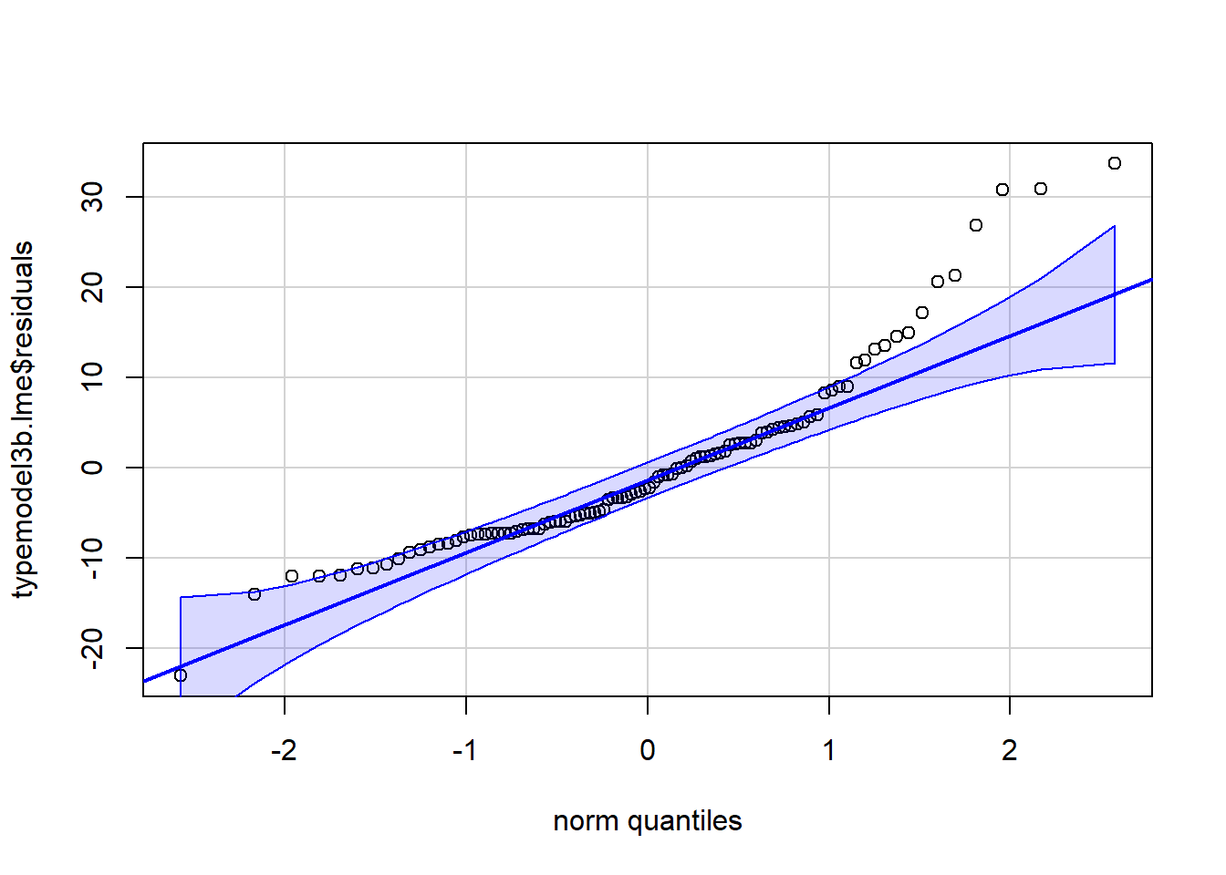
#hist(typemodel3b.lme$residuals)
#library(nortest)
#ad.test(typemodel3b.lme$residuals)
#plot(typemodel3b.lme$fitted,typemodel3b.lme$residuals)
5.4.1 Contrast evaluation from the alternative covariance structure model
We can return to the use of the testInteractions function and evaluate the same first orthogonal contrast employed above. But this time we will utilized the model that employed the unstructured covariance matrix specification. We see that the same -18.6 “psi” value is obtained again, but the test statistic value and the p value differ from the one seen above with the compound symmetry specification. This indicates a different set of residuals used in the lme model here. More exploration of how this test is constructed is warranted before usage can be recommended.
# phia may be able to work on these lme objects to obtain contrasts
#modmeans <- interactionMeans(fit2.lme)
#modmeans
#interactionMeans(fit2.lme, factors="type" )
# define first contrast on the rptd factor
ac1 <- list(type=c(4,-1,-1,-1,-1))
testInteractions(typemodel3b.lme, custom=ac1,adjustment="none")
## Chisq Test:
## P-value adjustment method: none
## Value Df Chisq Pr(>Chisq)
## type1 -18.6 1 7.6477 0.005684 **
## ---
## Signif. codes: 0 '***' 0.001 '**' 0.01 '*' 0.05 '.' 0.1 ' ' 15.5 Post hoc pairwise comparisons and planned/orthogonal contrasts
Although we have explored some attempts to evaluate contrasts in the sections above, using lme models, we broaden the perspective here.
If the analyst wants to perform post hoc pairwise comparison tests, it is also possible to pass the LMM object to the glht function from the multcomp package. This method employs a strategy not covered in class and is one that produces an approximate standard normal Z test statistic. By evaluating typemodel3b.lme, these tests employ standard errors based on the residual from that analysis where the covariance matrix was specified. The error rate inflation problem is addressed by using the Tukey correction method. Since the std errors vary from comparison to comparison, it is clear that one single error term is not employed, thus the errors are specific to the comparison.
library(multcomp)
multcomps <- glht(typemodel3b.lme, linfct = mcp(type = "Tukey"))
summary(multcomps)
##
## Simultaneous Tests for General Linear Hypotheses
##
## Multiple Comparisons of Means: Tukey Contrasts
##
##
## Fit: lme.formula(fixed = DV ~ type, data = rpt1.df, random = ~1 |
## snum, correlation = corSymm(form = ~1 | snum), method = "ML")
##
## Linear Hypotheses:
## Estimate Std. Error z value Pr(>|z|)
## homecage - clean == 0 -0.800 1.226 -0.653 0.93691
## iguana - clean == 0 0.500 1.906 0.262 0.99775
## whiptail - clean == 0 2.600 1.029 2.527 0.05872 .
## krat - clean == 0 16.300 4.734 3.443 0.00370 **
## iguana - homecage == 0 1.300 2.661 0.489 0.97676
## whiptail - homecage == 0 3.400 1.455 2.337 0.09325 .
## krat - homecage == 0 17.100 4.777 3.580 0.00206 **
## whiptail - iguana == 0 2.100 1.755 1.196 0.64880
## krat - iguana == 0 15.800 4.290 3.683 0.00135 **
## krat - whiptail == 0 13.700 3.962 3.458 0.00357 **
## ---
## Signif. codes: 0 '***' 0.001 '**' 0.01 '*' 0.05 '.' 0.1 ' ' 1
## (Adjusted p values reported -- single-step method)The ghlt function is also capable of evaluating a set of user-specified contrasts of any kind. Here, I created a matrix of our standard set of orthogonal contrasts employed elsewhere in this document and passed them to the glht function based on the unstructured covariance matrix model. Note that the errors differ for the four contrasts and are specific. This may be the best alternative for evaluating these contrasts with this data set, starting with the best fit LMM model, although an emmeans approach is found below. Note that the “estimates” here are the correct values for the means of the four chosen contrasts that we have examined previously. The reason that these effects are tested using a Z test statistic, rather than a t, is not apparent - requires beter understanding of ghlt.
contr <- rbind("clean_vs_all" = c(4,-1,-1,-1,-1),
               "hc_vs_three" = c(0,3,-1,-1,-1),
               "krat_vs_lizards" = c(0, 0,-1, -1, 2),
               "iguana_vs_whiptail" = c(0,0,1,-1,0))
multcontrasts.lmm <- glht(typemodel3b.lme, linfct = mcp(type = contr))
summary(multcontrasts.lmm)
##
## Simultaneous Tests for General Linear Hypotheses
##
## Multiple Comparisons of Means: User-defined Contrasts
##
##
## Fit: lme.formula(fixed = DV ~ type, data = rpt1.df, random = ~1 |
## snum, correlation = corSymm(form = ~1 | snum), method = "ML")
##
## Linear Hypotheses:
## Estimate Std. Error z value Pr(>|z|)
## clean_vs_all == 0 -18.600 6.726 -2.765 0.0180 *
## hc_vs_three == 0 -21.800 7.672 -2.841 0.0139 *
## krat_vs_lizards == 0 29.500 8.069 3.656 <0.001 ***
## iguana_vs_whiptail == 0 -2.100 1.755 -1.196 0.5053
## ---
## Signif. codes: 0 '***' 0.001 '**' 0.01 '*' 0.05 '.' 0.1 ' ' 1
## (Adjusted p values reported -- single-step method)5.5.1 Use of emmeans on the lme model
It is worth noting that emmeans can also perform its many capabilities on a lme model object. Here, we find that the t-tests are based on 36 df, implying use of some omnibus residual term. The t values do not match the univariate approach in chap 4 when emmeans was employed for the aov model object and they do not match those found from the initial lme approach, so the altered covariance stucture object produced different residuals. It is not clear how the concept of a “specific” error term fits into the linear mixed effects modeling framework.
fit3b.lme.emm <- emmeans(typemodel3b.lme, "type", data=rpt1.df)
lincombslme <- contrast(fit3b.lme.emm,
               list(type1=c(4, -1,-1,-1,-1),
                    type2=c(0,  3, -1, -1, -1),
                    type3=c(0,  0, -1, -1,  2),
                    type4=c(0,  0, -1,  1,  0)
                    ))
test(lincombslme, adjust="none")
## contrast estimate SE df t.ratio p.value
## type1 -18.6 7.09 36 -2.624 0.0127
## type2 -21.8 8.09 36 -2.696 0.0106
## type3 29.5 8.51 36 3.468 0.0014
## type4 2.1 1.85 36 1.135 0.2639
##
## Degrees-of-freedom method: containment