Chapter 12 A Larger Design and Trend Analysis
In order to expand the 1way ANOVA illustrations in this document, this chapter uses a different data set that permits implementation of trend analysis and incorporates an unequal sample size design. The data set comes from a laboratory study of ethanol effects on behavioral activity of mice (Data from B. Dudek). It is a dose-response study that is a completely randomized design with four doses of alcohol plus a control group. This chapter does a full analysis of this data set, employing many of the methods outlined in earlier chapters. Evaluation of the shape of the does response function is addressed with the use of Orthogonal Polynomial contrasts.
12.1 Import and process the data
In this data set, the DV is average mouse running speed (cm/sec, called speed15) in a fifteen minute test in an enclosed activity monitoring apparatus. The independent variable is called dose and has five levels: saline/control, 1.0, 1.5, 2.0, and 2.5 g/kg ethanol doses. The expectation was that lower doses would dis-inhibit behavior (more/faster running in the test apparatus) and then higher doses would begin to depress or sedate behavior, producing a biphasic dose response function. Total sample size was N=234 mice randomly assigned to the five conditions.
# read data from mouse alcohol/activity data set used earlier for the SPSS illustration
# data file is mouse_alcohol_doseresponse2b.csv
#mouse <- read.csv(file.choose(), stringsAsFactors=T)
mouse <- read.csv("data/mouse_alcohol_doseresponse2b.csv", stringsAsFactors = TRUE)
str(mouse)
## 'data.frame': 234 obs. of 2 variables:
## $ dose : Factor w/ 5 levels "1 g/kg","1.5 g/kg",..: 5 1 5 1 3 3 3 3 4 5 ...
## $ speed15: num 9.76 13.35 10.72 13.56 14.22 ...head(mouse)## dose speed15
## 1 SALINE 9.762282
## 2 1 g/kg 13.351472
## 3 SALINE 10.724117
## 4 1 g/kg 13.560831
## 5 2 g/kg 14.222366
## 6 2 g/kg 15.052335The characteristics of the “dose” variable create an issue for use as a factor in aov and lm models. This is because the nominal labels are alphabetically ordered and the control group is the last in that order (numbers come first in alphabetical ordering)
levels(mouse$dose)## [1] "1 g/kg" "1.5 g/kg" "2 g/kg" "2.5 g/kg" "SALINE"This ordering is not relevant for finding the omnibus F test in the aov or lm models but it will create a problem for evaluation of the trend components which will assume increasing order of the levels. Those levels were zero (called saline), 1, 1.5, 2, and 2.5 g/kg. We can change the order of those levels for the dose factor with the ordered function. This will enable proper use of the contr.poly specification for trend contrasts.
# force dose to be an ordered factor so that plots and tables maintain
# the correct order of the levels
mouse$dose <- ordered(mouse$dose,
                    levels=c("SALINE","1 g/kg","1.5 g/kg","2 g/kg","2.5 g/kg"))
levels(mouse$dose)
## [1] "SALINE" "1 g/kg" "1.5 g/kg" "2 g/kg" "2.5 g/kg"The original code for dose as a nominal variable/factor also creates problems for drawing line graphs with dose as the X axis variable. So, a new variable, “edose” is created to be explicitly numeric.
# create a new variable that is the quantitative scale that dose is expressed on
# this will be needed to draw line graphs
mouse[which(mouse$dose == "SALINE"),"edose"] <- 0
mouse[which(mouse$dose == "1 g/kg"),"edose"] <- 1
mouse[which(mouse$dose == "1.5 g/kg"),"edose"] <- 1.5
mouse[which(mouse$dose == "2 g/kg"),"edose"] <- 2
mouse[which(mouse$dose == "2.5 g/kg"),"edose"] <- 2.5
class(mouse$edose)
## [1] "numeric"The attach function is used to simplify our code even though current best practices in R recommend against using it. The downside of using it is not encountered in the illustrations in this chapter. It makes code for the graphing functions simpler.
attach(mouse)12.2 Exploratory Data Analysis: Numeric Summaries
Characteristics of the data set are initially explored with the describeBy function from psych. We can see that the sample sizes per group are nearly equal. One additional characteristic should be noted from this table. The standard deviations (and thus the variances) of the five groups differ over two-fold. Close examination of the homogeneity assumption will further evalauate this pattern.
# obtain descriptive statistics on the three groups using the psych package
require(psych)
tab1 <- describeBy(speed15,dose,mat=T, digits=3,type=2)
row.names(tab1) <- NULL
gt(tab1[2:15])| group1 | vars | n | mean | sd | median | trimmed | mad | min | max | range | skew | kurtosis | se |
|---|---|---|---|---|---|---|---|---|---|---|---|---|---|
| SALINE | 1 | 46 | 11.373 | 1.592 | 11.191 | 11.296 | 1.255 | 8.477 | 15.319 | 6.842 | 0.493 | 0.344 | 0.235 |
| 1 g/kg | 1 | 47 | 14.576 | 1.906 | 13.824 | 14.420 | 1.429 | 11.539 | 19.826 | 8.288 | 0.861 | 0.298 | 0.278 |
| 1.5 g/kg | 1 | 47 | 15.296 | 1.963 | 15.442 | 15.320 | 2.182 | 10.824 | 18.960 | 8.136 | -0.185 | -0.597 | 0.286 |
| 2 g/kg | 1 | 47 | 15.629 | 1.832 | 15.766 | 15.649 | 1.499 | 10.735 | 20.594 | 9.858 | -0.060 | 1.327 | 0.267 |
| 2.5 g/kg | 1 | 47 | 13.116 | 3.487 | 13.422 | 13.098 | 4.711 | 6.997 | 20.088 | 13.091 | 0.021 | -1.156 | 0.509 |
12.3 Exploratory Data Analysis: Graphical exploration
A line graph with standard error bars is the expected summary figure for evaluation of dose-response curves. Note that the code uses the “edose” variable that is numerically coded rather than the original “dose” variable.
# draw line graph using sciplot package
# difficult to get correct line graph with other R functions
# plotmeans and plotCI give nice graphs but X axis is not scaled as continuous
# lineplot.CI defaults to using std error bars, and the X axis is scaled properly
# error bars could be switched to CI's if desired.  See the help function on lineplot.CI
lineplot.CI(edose,speed15,x.cont=T,
            xlab="Ethanol Dose, g/kg",
            ylab="Running Speed, cm/sec",
            ylim=c(7,15.99))
# add axis break to indicate truncated axis
# axis.break, in the plotrix package, can add a double slaxh or zigzag
#    axis break indicator to any open plot
library(plotrix)
axis.break(2,7,style="zigzag")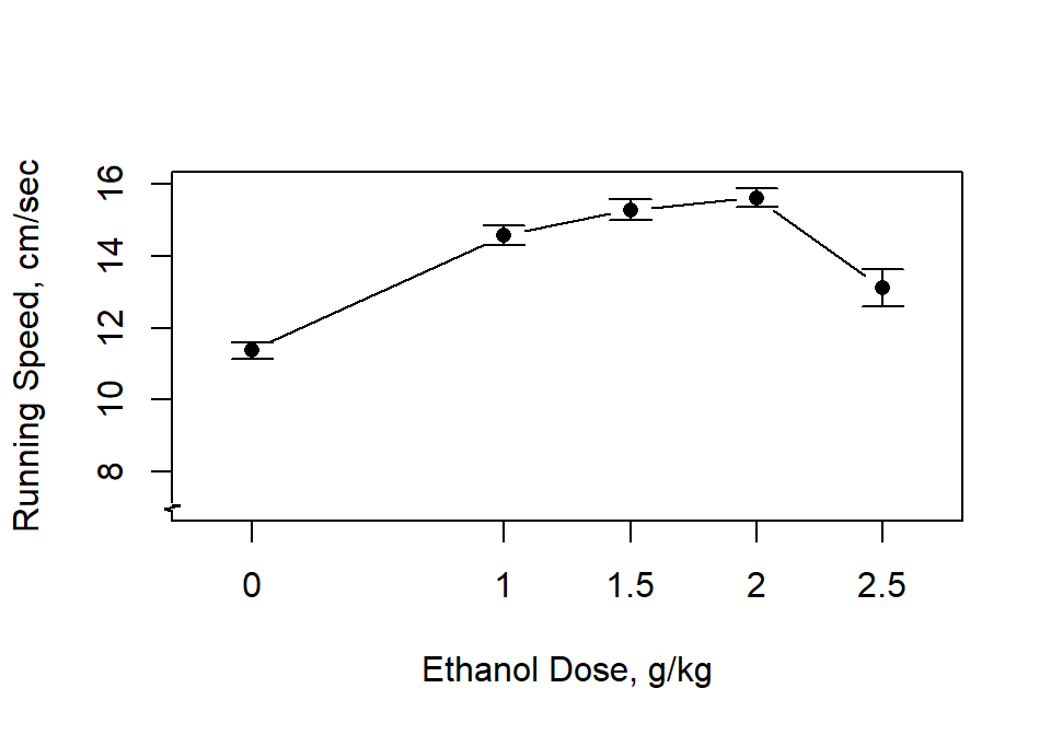
A boxplot can also be informative. The numeric “edose” variable is not needed here since the X axis in the box plot is not scaled. Recall that the correct ordering of levels of the dose variable occur because of the reording done above.
boxplot(speed15~dose,ylab="Running Speed, cm/sec",xlab=("Ethanol Dose, g/kg"))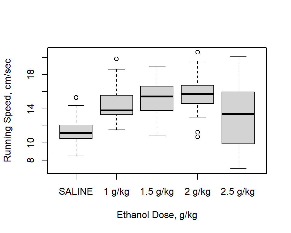
The ggplot2 package provides capabilities to produce plots that are publication quality. For the type of graph desired here, a line graph with Std Error bars, it takes some work to generate the plot. The ggplot function will not permit drawing the line graph of means +/- SEM’s directly from the data frame containing the raw data. Instead, a new data frame must be created, containing the summary statistics for each group. This is done with the summarySE function from the Rmisc package. Once created, the summary data frame can be used by ggplot. Here, we use the “edose” variable since it is a numeric variable.
mouse_summ <- Rmisc::summarySE(mouse,measurevar="speed15", groupvars="edose")
#str(mouse_summ)
# rename the column that contains the mean to something more less confusing
colnames(mouse_summ) <- c("edose", "N", "mean", "sd", "se", "95%ci" )
kable(mouse_summ)| edose | N | mean | sd | se | 95%ci |
|---|---|---|---|---|---|
| 0.0 | 46 | 11.37323 | 1.592286 | 0.2347698 | 0.4728507 |
| 1.0 | 47 | 14.57600 | 1.905680 | 0.2779720 | 0.5595286 |
| 1.5 | 47 | 15.29618 | 1.962592 | 0.2862734 | 0.5762384 |
| 2.0 | 47 | 15.62853 | 1.831644 | 0.2671728 | 0.5377909 |
| 2.5 | 47 | 13.11634 | 3.487325 | 0.5086786 | 1.0239169 |
The critical elements in creating the ggplot graph are the first line, the geom_line specification and the geom_errorbar specification. The remaining code controls text attributes and aesthetic properties of the graph. Note that in the ggplot figure, there is not a simple way to give the visual indicator that the Y axis has a break - the axis.break function does not work in the ggplot environment. The break symbols could be manually added, but I didn’t do that work here.
# now draw the plot
#win.graph() # or quartz() or x11()
ggplot(mouse_summ, aes(x=edose, y=mean)) +
  expand_limits(y=c(5,18)) +
  expand_limits(x=c(0,2.5)) +
  scale_y_continuous(breaks=0:4*4) +
  scale_x_continuous(breaks=0:5*.5) +
  geom_line() + geom_point(size=2) +
  geom_errorbar(aes(ymin=mean-se, ymax=mean+se), colour="black", width=.1)+
  xlab("Ethanol Dose (g/kg)")+
  ylab("Mean Running Speed (cm/sec)")+
  ggtitle("Alcohol Effects on Mouse Activity")+
  theme_classic()+
  theme(text = element_text(size=16))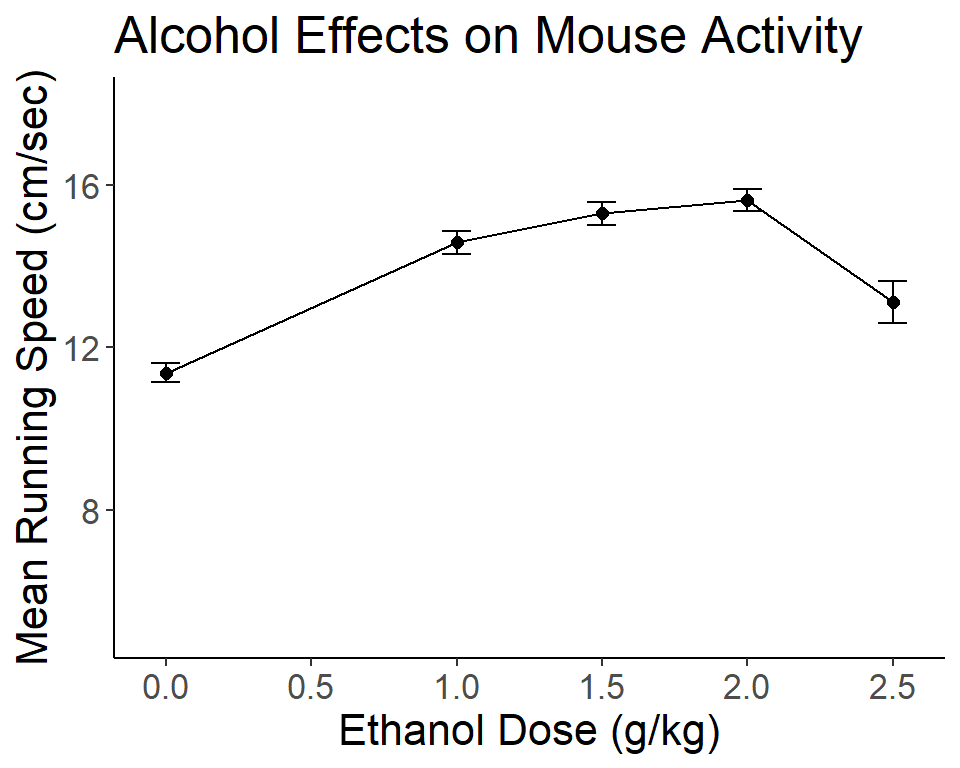
# code for bare minimum drawing of the line graph
#ggplot(mouse_summ, aes(x=edose, y=mean)) +
#  geom_line() +
#  geom_errorbar(aes(ymin=mean-se, ymax=mean+se), colour="black", width=.1)
12.4 Fit the base 1way aov model
The aov and lm functions require use of factors as IVs when performing analyses of variance. Therefore, the original “dose” variable is used throughout. It is important that we ordered the levels of that factor so that the orthononal polynomial trend contrasts properly match the levels.
First, we fit the base omnibus mode.
# fit basic analysis of variance model using aov
fit1t.aov <- aov(speed15~dose, data=mouse)
#summary(fit1.aov)
anova(fit1t.aov)
## Analysis of Variance Table
##
## Response: speed15
## Df Sum Sq Mean Sq F value Pr(>F)
## dose 4 573.28 143.321 28.002 < 2.2e-16 ***
## Residuals 229 1172.08 5.118
## ---
## Signif. codes: 0 '***' 0.001 '**' 0.01 '*' 0.05 '.' 0.1 ' ' 1# to show that for a 1way design, SS TYPE changes don't
# affect the omnibus BG SS
Anova(fit1t.aov,type=3) ## Anova Table (Type III tests)
##
## Response: speed15
## Sum Sq Df F value Pr(>F)
## (Intercept) 45848 1 8957.719 < 2.2e-16 ***
## dose 573 4 28.002 < 2.2e-16 ***
## Residuals 1172 229
## ---
## Signif. codes: 0 '***' 0.001 '**' 0.01 '*' 0.05 '.' 0.1 ' ' 112.5 Find the effect size indicators for the dose effect.
Initially, use the anova_stats function to obtain several effect size indicators.
anova_stats(fit1t.aov)## term | df | sumsq | meansq | statistic | p.value | etasq | partial.etasq | omegasq | partial.omegasq | epsilonsq | cohens.f | power
## ---------------------------------------------------------------------------------------------------------------------------------------------
## dose | 4 | 573.283 | 143.321 | 28.002 | < .001 | 0.328 | 0.328 | 0.316 | 0.316 | 0.317 | 0.699 | 1
## Residuals | 229 | 1172.080 | 5.118 | | | | | | | | |Next, use the etaSquared function from lsr.
#library(lsr)
#etaSquared(fit.1, type=1)
#etaSquared(fit.1, type=2)
etaSquared(fit1t.aov, type=3)
## eta.sq eta.sq.part
## dose 0.3284605 0.328460512.6 Implement orthogonal trend analysis
Once we learn how to create the orthogonal polynomial trend coefficients, we can use the same method as previously seen with the Hays data set to obtain SS and tests of those contrasts, using ‘split’ inside the summary function. Or we can use the summary.lm function. Fortunately, R has a built-in capability for orthogonal polynomials with the contr.poly function. It also permits exact specification of the numerical levels/spacing of the IV in the instance where levels of the quantitative IV are not equally spaced (as is our case here).
# now create the contrasts for trend analysis
# we need to define the contrasts based on an IV that
# has unequally spaced intervals
# by using the contr.poly function
# 5 levels with the IV values listed here
contrasts.dose <- contr.poly(5,scores=c(0,1,1.5,2,2.5))
contrasts(dose) <- contrasts.dose
contrasts(dose)
## .L .Q .C ^4
## SALINE -0.72782534 0.4907292 -0.1676525 0.03671115
## 1 g/kg -0.20795010 -0.4728845 0.6311625 -0.36711155
## 1.5 g/kg 0.05198752 -0.4595010 -0.2169621 0.73422310
## 2 g/kg 0.31192515 -0.1159905 -0.6213006 -0.55066732
## 2.5 g/kg 0.57186277 0.5576469 0.3747527 0.14684462Parenthetically, note that if the levels of the dose variable were equally spaced the could could simply have been the following. The contr.poly specifier does not even require parentheses in this case.
# code not used since the levels in our illustration were not equally spaced.
contrasts.dose <- contr.poly
contrasts(dose) <- contrasts.dose
contrasts(dose)
Next, we can fit the omnibus model again and then partition the trend SS and F tests inside the summary function. This time, the orthogonal polynomial trend coefficients will be used for the contrasts and tests of those contrasts will be provided using the split argument. Caution: This example data set has unequal sample sizes, so these F tests are tests of TYPE I SS.
# note:  summary with split on an aov object yields type I SS
# for these F tests
# use summary.lm, as below, to obtain Type III tests on either an
# aov object or directly on an lm object with summary.
fit2t.aov <- aov(speed15~dose)
summary(fit2t.aov,
        split=list(dose=list(linear=1, quadratic=2, cubic=3,quartic=4)))
## Df Sum Sq Mean Sq F value Pr(>F)
## dose 4 573.3 143.3 28.002 < 2e-16 ***
## dose: linear 1 157.7 157.7 30.808 7.85e-08 ***
## dose: quadratic 1 377.1 377.1 73.679 1.42e-15 ***
## dose: cubic 1 31.6 31.6 6.175 0.0137 *
## dose: quartic 1 6.9 6.9 1.345 0.2473
## Residuals 229 1172.1 5.1
## ---
## Signif. codes: 0 '***' 0.001 '**' 0.01 '*' 0.05 '.' 0.1 ' ' 1The alternative approach to providing inferences on the aov model object is to use the summary.lm function. This will produce t-tests, but they are equivalent to Type III SS F tests. Note that the squares of the t values do not exactly equal the F values produced above by the split argument in summary because of this Type I vs Type III distinction.
# or
summary.lm(fit2t.aov)
##
## Call:
## aov(formula = speed15 ~ dose)
##
## Residuals:
## Min 1Q Median 3Q Max
## -6.1194 -1.4152 -0.0894 1.3701 6.9716
##
## Coefficients:
## Estimate Std. Error t value Pr(>|t|)
## (Intercept) 13.9981 0.1479 94.645 < 2e-16 ***
## dose.L 1.8621 0.3319 5.610 5.80e-08 ***
## dose.Q -2.8387 0.3309 -8.580 1.45e-15 ***
## dose.C -0.8203 0.3301 -2.485 0.0137 *
## dose^4 -0.3827 0.3300 -1.160 0.2473
## ---
## Signif. codes: 0 '***' 0.001 '**' 0.01 '*' 0.05 '.' 0.1 ' ' 1
##
## Residual standard error: 2.262 on 229 degrees of freedom
## Multiple R-squared: 0.3285, Adjusted R-squared: 0.3167
## F-statistic: 28 on 4 and 229 DF, p-value: < 2.2e-16Alternatively, we can do the trend analysis with lm and obtain the parameter estimates instead of variance partitioning as was the case with applying summary.lm to the aov object. Note that the orthogonal polynomial contrasts are still in effect from above. The results produce t values that are close, but not identical, to the square roots of the F tests seen just above but they match the t values from summary.lm. If the design has equal sample size then these three different ways of obtaining inferences on the contrasts will all match.
fit3t.lm <- lm(speed15~dose)
summary(fit3t.lm)
##
## Call:
## lm(formula = speed15 ~ dose)
##
## Residuals:
## Min 1Q Median 3Q Max
## -6.1194 -1.4152 -0.0894 1.3701 6.9716
##
## Coefficients:
## Estimate Std. Error t value Pr(>|t|)
## (Intercept) 13.9981 0.1479 94.645 < 2e-16 ***
## dose.L 1.8621 0.3319 5.610 5.80e-08 ***
## dose.Q -2.8387 0.3309 -8.580 1.45e-15 ***
## dose.C -0.8203 0.3301 -2.485 0.0137 *
## dose^4 -0.3827 0.3300 -1.160 0.2473
## ---
## Signif. codes: 0 '***' 0.001 '**' 0.01 '*' 0.05 '.' 0.1 ' ' 1
##
## Residual standard error: 2.262 on 229 degrees of freedom
## Multiple R-squared: 0.3285, Adjusted R-squared: 0.3167
## F-statistic: 28 on 4 and 229 DF, p-value: < 2.2e-1612.7 Effect size proportion of variance estimates for contrasts.
A manual approach is used since I am still looking for an efficient way to generate effect size estimates for analytical contrasts. Find SStotal to be used as the denominator for eta squared computations for each contrast. Then create a vector of the SS for those four trend components. Then Divide the vector by SStotal for the four eta squared estimates.
A second useful descriptive statistic takes each trend component SS and divides by the SSbetween. This yields a proportion statistic that characterizes the percentage of the between-group effect that each orthogonal trend component accounts for. I used the SS values from the summary function application to the aov object.
# first define SStotal
sst <- var(speed15)*(length(speed15)-1)
sst
## [1] 1745.362#Then create a vector of the SS components for trend
sstrend <- c(157.7,377.1,31.6,6.9)
names(sstrend) <- c("linear", "quadratic", "cubic", "quadratic")
sstrend## linear quadratic cubic quadratic
## 157.7 377.1 31.6 6.9sstrend/sst## linear quadratic cubic quadratic
## 0.090353733 0.216058293 0.018105123 0.003953334sstrend/573.3## linear quadratic cubic quadratic
## 0.27507413 0.65777080 0.05511948 0.0120355812.8 using emmeans for trend analysis
In order to use emmeans to perform the orthogonal trend decomposition, we need to be able to pass the exact trend coefficients that we saw earlier. Since they were based on unequally spaced intervals and since R chooses a scale such that the sum of the squared coefficients equals 1 (orthonormalizing), the coefficients are decimal quantities. For accuracy we need to extract those exact values from the contrasts(dose) object and then pass them to the emmeans function. Initially, these coefficients are in a matrix, and I found it easier to convert that matrix to a dataframe so that the columns of coefficients can be extracted. Notice the possibility of adjusting the pvalues and/or CIs for the multiple testing situation. Just for demonstration, I did not adjust the t-test inferences but I did adjust the CIs (just to show how the adjustment is done).
fit2.emm.a <- emmeans(fit3t.lm, "dose", data=mouse)
trend <- as.data.frame(contrasts(mouse$dose))
# check with, e.g., trend[,4]
lincombs <- contrast(fit2.emm.a,
               list(linear=trend$.L,
                    quadratic=trend$.Q,
                    cubic=trend$.C,
                    quartic=trend$'^4'
                    ))
test(lincombs, adjust="none")
## contrast estimate SE df t.ratio p.value
## linear 1.435 0.331 229 4.331 <.0001
## quadratic -3.158 0.331 229 -9.541 <.0001
## cubic -0.114 0.330 229 -0.346 0.7293
## quartic -0.544 0.330 229 -1.648 0.1007confint(lincombs, adjust="sidak")## contrast estimate SE df lower.CL upper.CL
## linear 1.435 0.331 229 0.603 2.267
## quadratic -3.158 0.331 229 -3.990 -2.327
## cubic -0.114 0.330 229 -0.944 0.715
## quartic -0.544 0.330 229 -1.373 0.285
##
## Confidence level used: 0.95
## Conf-level adjustment: sidak method for 4 estimatesThese t test values match the lm model output (and application of summary.lm to the aov object) where regression coefficients were tested and thus relate to Type III SS. This is probably the most appropriate way to do trend analysis when there is unequal N, although it is more cumbersome than using the “split” argument.
12.9 Summary to this point in the analysis of the dose response data set
At this point, we have information from the analysis that largely fits what our eye saw from the dose response curve figures. Low doses tended to increase running speed relative to the control condition but at the highest dose, the curve began to take a downward trajectory, reflecting the expectation outlined above. In terms of the trend analysis, the shape of the curve was largely influenced by linear and quadratic components, with the quadratic bend accounting for the majority of the Between group effect of the IV (the 66% value just calculated).
12.10 Post Hoc tests
The full ANOVA and trend decomposition didn’t tell us about one interesting question that emerges from examination of the dose response curve. We might as whether the 2.5 dose mean is actually different from the 2.0 dose. I.e., is the drop “significant”. This is explicitly a post hoc question. The most direct way of evaluating this is with a Tukey test. I’ll opt for doing both the standard Tukey HSD test and the DTK test here. DTK is applicable when there is unequal sample size and heterogeneity of variance (we had a hint of that when we examined the sd’s for the five groups). Since that one pairwise comparison (2 vs 2.5) was derived from visual examination of the figure in a post hoc way, it can be argued that all pairwise comparisons were visually taken in to account. The results of the DTK test function will evaluate all of those pairwise comparisons and the alpha rate adjustment properly takes this into account.
# first, use the Tukey HSD test procedure
TukeyHSD(fit1t.aov)
## Tukey multiple comparisons of means
## 95% family-wise confidence level
##
## Fit: aov(formula = speed15 ~ dose, data = mouse)
##
## $dose
## diff lwr upr p adj
## 1 g/kg-SALINE 3.2027633 1.9125852 4.4929414 0.0000000
## 1.5 g/kg-SALINE 3.9229500 2.6327718 5.2131281 0.0000000
## 2 g/kg-SALINE 4.2552967 2.9651186 5.5454748 0.0000000
## 2.5 g/kg-SALINE 1.7431045 0.4529263 3.0332826 0.0023542
## 1.5 g/kg-1 g/kg 0.7201867 -0.5630363 2.0034096 0.5355178
## 2 g/kg-1 g/kg 1.0525334 -0.2306895 2.3357563 0.1634975
## 2.5 g/kg-1 g/kg -1.4596588 -2.7428818 -0.1764359 0.0168655
## 2 g/kg-1.5 g/kg 0.3323467 -0.9508762 1.6155697 0.9535766
## 2.5 g/kg-1.5 g/kg -2.1798455 -3.4630685 -0.8966226 0.0000500
## 2.5 g/kg-2 g/kg -2.5121922 -3.7954152 -1.2289693 0.0000018# now request the Dunnett-Tukey-Kramer test:
DTK.result <- DTK.test(speed15,edose)
DTK.result## [[1]]
## [1] 0.05
##
## [[2]]
## Diff Lower CI Upper CI
## 1-0 3.2027633 2.16944629 4.2360803
## 1.5-0 3.9229500 2.87151157 4.9743884
## 2-0 4.2552967 3.24521665 5.2653768
## 2.5-0 1.7431045 0.15203497 3.3341740
## 1.5-1 0.7201867 -0.41301751 1.8533909
## 2-1 1.0525334 -0.04240628 2.1474731
## 2.5-1 -1.4596588 -3.10589543 0.1865778
## 2-1.5 0.3323467 -0.77974361 1.4444370
## 2.5-1.5 -2.1798455 -3.83756613 -0.5221249
## 2.5-2 -2.5121922 -4.14361391 -0.8807706#DTK.plot(DTK.result)Of course there other ways to do post hoc testing that could fit this data set. We might want to use the Dunnett test to compare each treatment group with control. It turns out that none of the four CIs overlaps zero, so we conclude each dose significantly raised DV scores.
### The DUNNETT TYPE OF TEST FOR COMPARING TREATMENTS TO A COMMON CONTROL GROUP
require(multcomp)
fit1.dunnett <- glht(fit1t.aov,linfct=mcp(dose="Dunnett"))
# obtain CI's do test each difference
confint(fit1.dunnett, level = 0.95)
##
## Simultaneous Confidence Intervals
##
## Multiple Comparisons of Means: Dunnett Contrasts
##
##
## Fit: aov(formula = speed15 ~ dose, data = mouse)
##
## Quantile = 2.4576
## 95% family-wise confidence level
##
##
## Linear Hypotheses:
## Estimate lwr upr
## 1 g/kg - SALINE == 0 3.2028 2.0496 4.3559
## 1.5 g/kg - SALINE == 0 3.9229 2.7698 5.0761
## 2 g/kg - SALINE == 0 4.2553 3.1022 5.4084
## 2.5 g/kg - SALINE == 0 1.7431 0.5900 2.8962We might also wish to do pairwise comparisons with methods other than the Tukey or DTK test. We can use the pairwise.t.test function.
# This function provides several of the bonferroni style corrections
# for pairwise multiple comparisons.  Note that it permits use of
# the pooled within cell variance as the core error term.
# first, just do pairwise comparisons with bonferroni corrections for
# having done a set of three "contrasts".  should match results seen
# above in the BonferroniCI function.
pairwise.t.test(speed15,dose,pool.sd=TRUE,p.adj="bonf")
##
## Pairwise comparisons using t tests with pooled SD
##
## data: speed15 and dose
##
## SALINE 1 g/kg 1.5 g/kg 2 g/kg
## 1 g/kg 7.8e-10 - - -
## 1.5 g/kg 6.1e-14 1.0000 - -
## 2 g/kg 5.6e-16 0.2506 1.0000 -
## 2.5 g/kg 0.0026 0.0199 5.1e-05 1.8e-06
##
## P value adjustment method: bonferroni# We can change the approach to the Holm, Hochberg, Hommel,
# Benjamini and Hochberg, Benjamini&Yekutieli, and fdr corrections,
# as well as "none" which will give the same thing as the LSD test.
# Choice of these depends on several factors, including whether
# the contrasts examined are independent (and they are not since they
# are all of the pairwise comparisons,
# Of these modified bonferroni type of approaches, the "BY" and "fdr"
# approaches are probably the most appropriate here, since some of our
# comparisons are correlated and BY permits that correlation to be either
# positive or negative
#pairwise.t.test(dv,factora,pool.sd=TRUE,p.adj="holm")
#pairwise.t.test(dv,factora,pool.sd=TRUE,p.adj="hochberg")
#pairwise.t.test(dv,factora,pool.sd=TRUE,p.adj="hommel")
#pairwise.t.test(dv,factora,pool.sd=TRUE,p.adj="BH")
pairwise.t.test(speed15,dose,pool.sd=TRUE,p.adj="BY")##
## Pairwise comparisons using t tests with pooled SD
##
## data: speed15 and dose
##
## SALINE 1 g/kg 1.5 g/kg 2 g/kg
## 1 g/kg 7.6e-10 - - -
## 1.5 g/kg 8.9e-14 0.4041 - -
## 2 g/kg 1.6e-15 0.0917 1.0000 -
## 2.5 g/kg 0.0012 0.0083 3.0e-05 1.3e-06
##
## P value adjustment method: BYpairwise.t.test(speed15,dose,pool.sd=TRUE,p.adj="fdr")##
## Pairwise comparisons using t tests with pooled SD
##
## data: speed15 and dose
##
## SALINE 1 g/kg 1.5 g/kg 2 g/kg
## 1 g/kg 2.6e-10 - - -
## 1.5 g/kg 3.0e-14 0.13796 - -
## 2 g/kg 5.6e-16 0.03132 0.47710 -
## 2.5 g/kg 0.00043 0.00284 1.0e-05 4.5e-07
##
## P value adjustment method: fdr#pairwise.t.test(dv,factora,pool.sd=TRUE,p.adj="none")
# note that setting pool.sd to FALSE changes the outcome since
# it employs a Welch or Fisher-Behrens type of approach
pairwise.t.test(speed15,dose,pool.sd=FALSE,p.adj="bonf")##
## Pairwise comparisons using t tests with non-pooled SD
##
## data: speed15 and dose
##
## SALINE 1 g/kg 1.5 g/kg 2 g/kg
## 1 g/kg 9.8e-13 - - -
## 1.5 g/kg < 2e-16 0.74370 - -
## 2 g/kg < 2e-16 0.07593 1.00000 -
## 2.5 g/kg 0.02771 0.14049 0.00372 0.00042
##
## P value adjustment method: bonferroni# or
pairwise.t.test(speed15,dose,pool.sd=FALSE,p.adj="fdr")##
## Pairwise comparisons using t tests with non-pooled SD
##
## data: speed15 and dose
##
## SALINE 1 g/kg 1.5 g/kg 2 g/kg
## 1 g/kg 3.3e-13 - - -
## 1.5 g/kg < 2e-16 0.08263 - -
## 2 g/kg < 2e-16 0.01085 0.39824 -
## 2.5 g/kg 0.00462 0.01756 0.00074 0.00011
##
## P value adjustment method: fdr12.11 Evaluation of Assumptions: graphical and inferential evaluation
Perhaps this section is placed too late in the flow of the analyses since violations of the assumption(s) would have implications for most of the tests above.
First, we can obtain the standard pair of plots for evaluating normality and homoscedasticity of the residuals from the ANOVAs done above. It is easiest to work with the lm fit object. The first plot reveals the heteroscedasticity that we suspected. The group that has the largest residual spread is the group that had a mean near 13 (the 2.5 g/kg dose group), and this group had the highest standard deviation, as seen with the initial descriptive statistics. The second plot, at first glance gives a reasonable impression of a fit to normality for the residuals but closer inspection suggests a pattern where the largest outliers deviate a bit from expectation.
plot(fit3t.lm,which=1)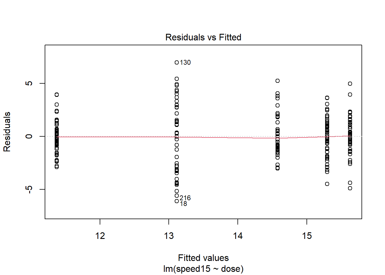
plot(fit3t.lm,which=2)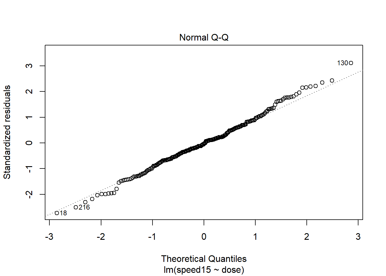
Lets pursue this potential non-normality a bit further. If we extract the residuals from the lm object, we can draw both the qqPlot figure and a frequency histogram.
qqPlot(fit3t.lm$residuals)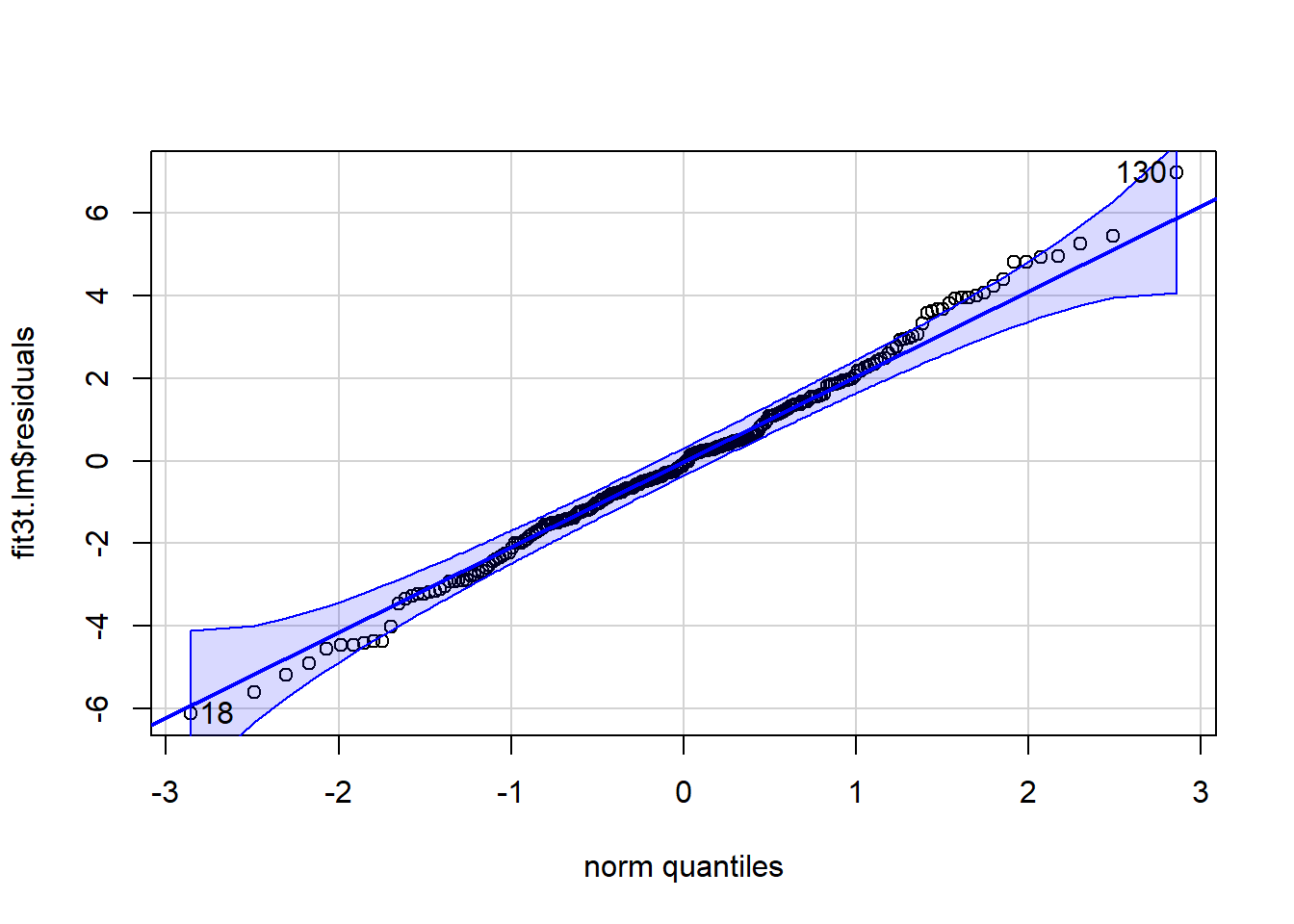
## [1] 130 18hist(fit3t.lm$residuals, prob=TRUE, col="gray82",breaks=16)
lines(density(fit3t.lm$residuals, bw=1))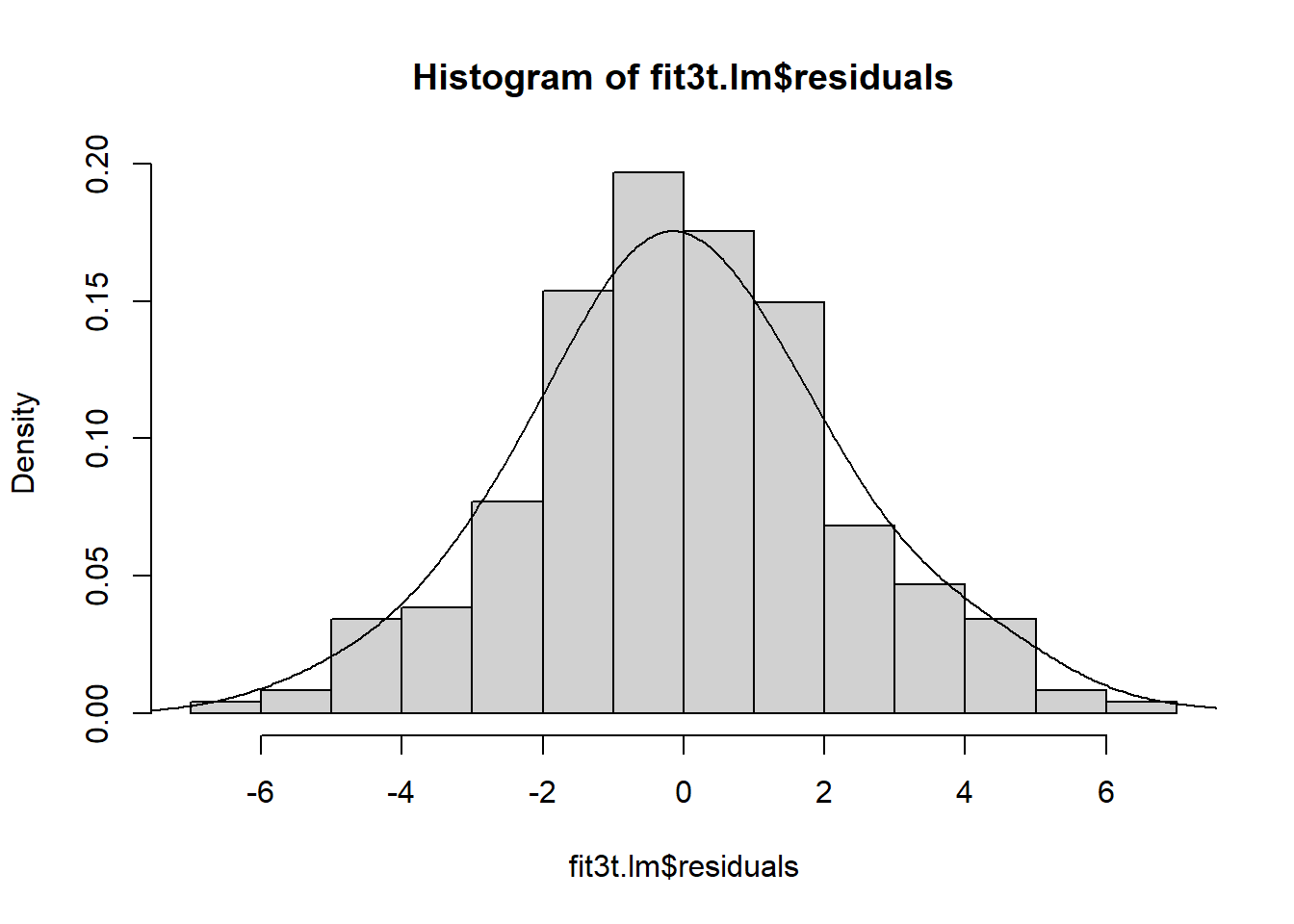
Both figures suggest that the normality assumption may not be violated here, but we can do a test. We find that the Anderson-Darling test does not permit rejection of the null hypothesis that normality is present.
#library(nortest)
ad.test(residuals(fit3t.lm)) #get Anderson-Darling test for normality (nortest package must be installed)
##
## Anderson-Darling normality test
##
## data: residuals(fit3t.lm)
## A = 0.42988, p-value = 0.3059Now let’s evaluate the Homogeneity of Variance Assumption. Among the several ways we reviewed to do this, the median-centered Levene test is probably adequate:
levene.test(speed15,edose,location="median")##
## Modified robust Brown-Forsythe Levene-type test based on the absolute
## deviations from the median
##
## data: speed15
## Test Statistic = 13.477, p-value = 7.011e-10##########################################
## Plot of cell means vs cell variances ##
##########################################
# recall that this type of plot helps evaluate whether
# heterogeneity of variance might have arisen from a simple
# scaling issue. If so, then scale transformations may help.
# E.g,, a postive mean-variance correlation reflects a situation where
# a log transformation or a fractional exponent transformation of the DV
# might produce homoscedasticity.
# I'm also using the tapply function here in ways that we have not covered.
# Tapply is an important function in dealing with factors.
plot(tapply(speed15, dose, mean), tapply(speed15, dose, var), xlab = "Cell Means",
ylab = "Cell Variances", pch = levels(edose))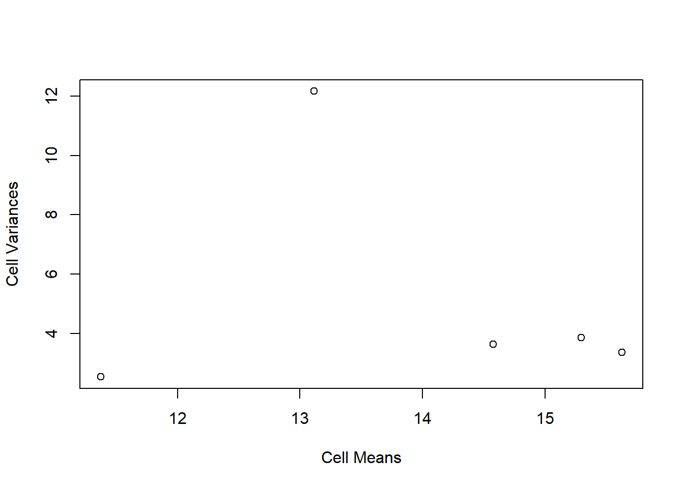
# examination of the plot shows that the heterogeneity is not simply due to a
# mean variance correlation.  the group with the highest variance is the highest
# dose group and no simple transformation can take care of the problem.
# the dispersion difference may come from a sex difference that was not examined here.
# thus the model may be underspecified and this may have produced the heterogeneity

#  recall that we can do the extension of the Welch test to 1-way anova
12.12 Alternate analyses when faced with Heteroscadisticity
The omnibus F test can be re-examined, using the Welch f test approach and we already reviewed that capability with the oneway.test function. Unsurprisingly, the omnibus F remains significant (with this large N design and strong treatment effects) at the .05 level.
oneway.test(speed15~dose,var.equal=F)##
## One-way analysis of means (not assuming equal variances)
##
## data: speed15 and dose
## F = 46.616, num df = 4.00, denom df = 113.58, p-value < 2.2e-16Wilcox argues for use of the percentile t approach to bootstrapping whenver either/or heteroscadisticy or non-normality are present. That method was simple to implement and also yields a rejection of the omnibus null hypothesis. The “tr” argument specifies the degree of trimming. This choice is not to be taken lightly and users should be familiar with the literature on trimmed means, Winsorized means, and other M-estimators. The abundant writings of Wilcox (e.g., (Wilcox, 2016)) are a good starting point.
# from the WRS2 package
t1waybt(speed15~edose,tr=.2,nboot=2000, data=mouse)
## Call:
## t1waybt(formula = speed15 ~ edose, data = mouse, tr = 0.2, nboot = 2000)
##
## Effective number of bootstrap samples was 2000.
##
## Test statistic: 49.8329
## p-value: 0
## Variance explained: 0.375
## Effect size: 0.613Pairwise comparisons using bootstrapping also yield similar conclusions to the traditional tests done above.
# from the WRS2 package
mcppb20(speed15~edose,tr=.2,nboot=2000, data=mouse)
## Call:
## mcppb20(formula = speed15 ~ edose, data = mouse, tr = 0.2, nboot = 2000)
##
## psihat ci.lower ci.upper p-value
## 0 vs. 1 -2.97790 -4.08606 -2.02812 0.000
## 0 vs. 2 -4.07103 -5.21790 -3.00591 0.000
## 0 vs. 2.5 -4.32550 -5.25236 -3.44927 0.000
## 0 vs. 1.5 -1.78139 -3.70158 0.26297 0.006
## 1 vs. 2 -1.09314 -2.22172 0.16915 0.019
## 1 vs. 2.5 -1.34761 -2.39651 -0.29189 0.001
## 1 vs. 1.5 1.19650 -0.72582 3.13702 0.081
## 2 vs. 2.5 -0.25447 -1.36754 0.86564 0.524
## 2 vs. 1.5 2.28964 0.47334 4.33964 0.000
## 2.5 vs. 1.5 2.54411 0.49023 4.60210 0.000I am not yet confident of a way to implement bootstrapping for analytical contrasts, such as trend analysis, in R. It should be possible to do it by bootstrapping the lm model fit. One approach is found in the Resampling chapter.