Chapter 6 Beginning to Explore the emmeans package for post hoc tests and contrasts

The emmeans package is one of several alternatives to facilitate post hoc methods application and contrast analysis. It is a relatively recent replacement for the lsmeans package that some R users may be familiar with. It is intended for use with a wide variety of ANOVA models, including repeated measures and nested designs where the initial modeling would employ ‘aov’, ‘lm’ ‘ez’ or ‘lme4’ (mixed models).

6.1 Using emmeans for pairwise post hoc multiple comparisons.

Initially, a minimal illustration is presented. First is a “pairwise” approach to followup comparisons, with a p-value adjustment equivalent to the Tukey test. The emmeans function requires a model object to be passed as the first argument. We could use either fit1 (the aov object) or fit2 (the lm object) originally created in the base ANOVA section of this document.

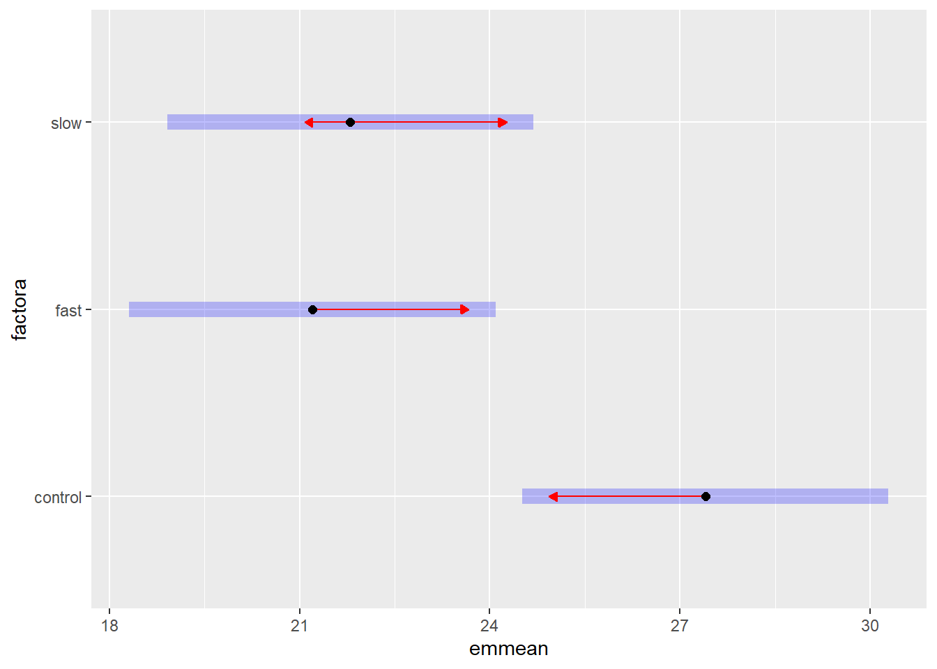
First, emmeans is used to extract a “grid” of group descriptive statistics including mean, SEM (based on the pooled error term), df, and upper and lower 95% CI values. That object can then be passed to either the pairs function for tests, or the plot function for graphing.

#library(emmeans)
# reminder: fit.2 <- lm(dv~factora, data=hays)
fit2.emm.a <- emmeans(fit.2, "factora", data=hays)
#fit2.emm.a
pairs(fit2.emm.a, adjust="tukey")

##  contrast       estimate   SE df t.ratio p.value
##  control - fast      6.2 1.99 27   3.113  0.0117
##  control - slow      5.6 1.99 27   2.811  0.0239
##  fast - slow        -0.6 1.99 27  -0.301  0.9513
## 
## P value adjustment: tukey method for comparing a family of 3 estimates

plot(fit2.emm.a, comparisons = TRUE)

#pairs(fit2.emm.a, adjust="none")

The blue bars on the plot are the confidence intervals. The red arrowed lines represent a scheme to determine homogeneous groups. If the red lines overlap for two groups, then they are not signficantly different using the method chosen.

The ‘adjust’ argument can take one of several useful methods. ‘tukey’ is default, but others including ‘sidak’, ‘bonferroni’, etc can be specified. Specifying ‘none’ produces unadjusted p-values. See help with ‘?emmeans::summary.emmGrid’ for details. Here is an example using the ‘holm’ method of adjustment.

library(emmeans)
fit2.emm.b <- emmeans(fit.2, "factora", data=hays)
pairs(fit2.emm.b, adjust="holm")

##  contrast       estimate   SE df t.ratio p.value
##  control - fast      6.2 1.99 27   3.113  0.0131
##  control - slow      5.6 1.99 27   2.811  0.0181
##  fast - slow        -0.6 1.99 27  -0.301  0.7655
## 
## P value adjustment: holm method for 3 tests

plot(fit2.emm.b, comparisons = TRUE)

#pairs(fit2.emm.a, adjust="none")

6.2 Analytical Contrasts

Next, we will create linear combination contrasts and test them. Notice that in “testing” the contrast, no alpha-rate control adjustments are made. This produces t-values that are the square root of the F’s we found above for the ‘split’ approach on ‘aov’ or the regression coefficient t values from ‘lm’ objects with ‘summary’. It is also possible to obtain confidence intervals on the contrasts, and I show how an adjustment can be done (but it wouldn’t make sense to adjust the CIs with one method and the tests with another. I show a commented test and confint functions to remind us that the adjustment could be applied. But the output is showing only unadjusted tests and CIs - appropriate if the set of contrasts is a priori.

Interpreting the scale of the estimates and CIs is potentially problematic. If they are in the scale of 2, -1, -1 and 0, 1, -1, they would produce the 11.8 and -.6 psi values we have seen several times previously for this data set. It is all well and good if the only thing we are using the CIs for is to evaluate whether they overlap zero (as a proxy for the hypothesis test). But the actual range of values is arbitrarily dependent on the values of the Coefficients (thus their variance). One strategy might be to implement what we saw in SPSS UNIANOVA. We could constrain the largest coefficient value to be a “1”, and use fractions for the remainder, when necessary. This would put the estimates and CI’s on a scale that fits the way we discuss the contrasts: Contrast 1 evaluates whether control differs from the average of fast and slow. The 5.9 estimate seen below is meaningful in this way of scaling the contrasts, and is half the 11.8 value seen with the 2, -1, -1 coefficients.

So a redo of the earlier approach to contrasts above could look like this using test function on the contrasts fit to the emm model grid of means:

lincombs <- contrast(fit2.emm.a,
               list(ac1=c(1,-.5,-.5), ac2=c(0,1,-1))) # second one not changed
test(lincombs, adjust="none")

##  contrast estimate   SE df t.ratio p.value
##  ac1           5.9 1.72 27   3.420  0.0020
##  ac2          -0.6 1.99 27  -0.301  0.7655

#test(lincombs, adjust="sidak")
confint(lincombs, adjust="none")

##  contrast estimate   SE df lower.CL upper.CL
##  ac1           5.9 1.72 27     2.36     9.44
##  ac2          -0.6 1.99 27    -4.69     3.49
## 
## Confidence level used: 0.95

#confint(lincombs, adjust="sidak")

To re-emphasize….. the psi value for the contrasts are directly related to how we speak about what the contrasts are evaluating. The mean of “control” is 5.9 units above the average of the “fast” and “slow” conditions. And for the second contrast, “fast” is .6 units below the mean of “slow”. In this scaling, the CIs are more directly interpretable at their edges. But make sure to note that the t values and p values do not change with this scaling change.

6.3 Concluding comments on emmeans

The emmeans package is a very powerful tool. But it is almost overkill for a one-way design. Its utility will become impressive for factorial between-groups designs, for repeated measures designs, and for linear mixed effect models. The goal is to revisit it with the first two of those three applications.