Chapter 13 Unequal Sample Sizes
The presence of unequal samples sizes has major implications in factorial designs that require care in choice of SS decomposition types (e.g., Type I vs II, vs III). For 1-way layouts, the impact is more minimal. However, there are some things to be aware of, particularly with regard to use of contrasts, and this chapter addresses those issues.
The critical starting point in understanding why the issue arises with contrasts (even “orthogonal” ones), is to know that when a design is unbalanced (unequal n’s), the coding vectors (when applied to all cases) are not completely uncorrelated. Thus the regression modeling is not clean. It has to cope with correlated IVs and this is where the Type I, II, and III SS issues come into play.
13.1 Import the data and Describe
We can use the same original data set from earlier parts of this tutorial, the “hays” data set. However, I randomly deleted five cases from that data set, two from the control group, one from the fast group, and three from the slow group. The data are in a .csv file that is read here.
hays_unbal <- read.csv("data/hays_unequal.csv",stringsAsFactors=TRUE)The descriptive statistics show that the three means differ a small amount from their original values in the equal-sample-size illustrations above, but not radically so.
describeBy(hays_unbal$dv, group=hays_unbal$factora, type=2)##
## Descriptive statistics by group
## group: control
## vars n mean sd median trimmed mad min max range skew kurtosis se
## X1 1 8 26.62 5.32 26.5 26.62 4.45 19 36 17 0.32 0.37 1.88
## ------------------------------------------------------------
## group: fast
## vars n mean sd median trimmed mad min max range skew kurtosis se
## X1 1 9 20.33 4.69 19 20.33 4.45 15 30 15 1.03 1.05 1.56
## ------------------------------------------------------------
## group: slow
## vars n mean sd median trimmed mad min max range skew kurtosis se
## X1 1 7 22.43 1.51 23 22.43 1.48 20 24 4 -0.62 -0.81 0.57We can visualize the data set with this multiple-panel graph produced in ggplot.
# Modeled after https://dmyee.files.wordpress.com/2016/03/advancedggplot.pdf
#Histograms of  DV by Shelf
#library("RColorBrewer")
cbPalette <- c("#999999", "#E69F00", "#56B4E9", "#009E73",
               "#F0E442", "#0072B2", "#D55E00", "#CC79A7")
p1<-ggplot(data = hays_unbal, aes(x = dv, fill=factora)) +
  geom_histogram(binwidth = .1) +
  scale_fill_manual(values=cbPalette) +
  #scale_fill_brewer(palette="Paired") +
  #scale_colour_grey() + scale_fill_grey() +
  xlab("Rating") + ylab("Count") +
  ggtitle("Histograms, by Factor A") +
  theme_minimal() +
  theme(plot.title = element_text(size=10, face = "bold", hjust = 1))

# Boxplots of "Healthiness" Rating" by factora
p2<-ggplot(data = hays_unbal, aes(x = factora, y = dv, fill=factora)) +
  geom_boxplot() +xlab("Factor A") + ylab("Rating") +
  scale_fill_manual(values=cbPalette) +
  #scale_fill_brewer(palette="Paired") +
  #scale_colour_grey() + scale_fill_grey() +
  ggtitle("Boxplots of DV by Factor A") +
  theme_minimal() +
  theme(plot.title = element_text(size=10, face = "bold", hjust = 1))

# Violin plots of "Healthiness" Rating" by factora
p3<-ggplot(data = hays_unbal, aes(x = factora, y = dv, fill=factora)) +
  geom_violin(alpha=.25, color="gray") +
  geom_jitter(alpha=.5, aes(color=factora), position=position_jitter(width=0.3)) +
  scale_fill_manual(values=cbPalette) + scale_colour_manual(values=cbPalette) +
  #scale_fill_brewer(palette="Paired") +
    #scale_colour_grey() + scale_fill_grey() +
  coord_flip() +
  xlab("Factor A") + ylab("DV") +
  ggtitle("Violin plots of DV by Shelf") +
  theme_minimal() +theme(plot.title = element_text(size=10, face = "bold", hjust = 1))

# Creating a matrix that defines the layout
# (not all graphs need to take up the same space)
lay <- rbind(c(1,2),c(3,3))# Plotting the plots on a grid
grid.arrange(p1, p2, p3, ncol=2, layout_matrix=lay)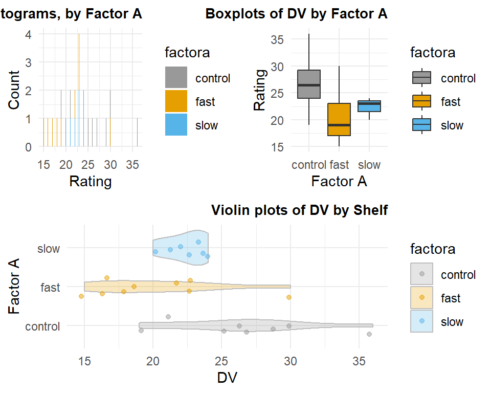
13.2 Fit the model with aov
The omnibus ANOVA model can be fit with aov in the previously defined manner, and an omnibus F test is returned.
fit1_unbal <- aov(dv~factora, data=hays_unbal)
anova(fit1_unbal)
## Analysis of Variance Table
##
## Response: dv
## Df Sum Sq Mean Sq F value Pr(>F)
## factora 2 171.37 85.685 4.6425 0.0214 *
## Residuals 21 387.59 18.457
## ---
## Signif. codes: 0 '***' 0.001 '**' 0.01 '*' 0.05 '.' 0.1 ' ' 1It is useful to recall that aov is a wrapper for the lm function and thus requires the IV to be a factor so that coding vectors (contrasts) can be produced. Let’s recall what the default contrasts are for a factor. The are dummy or indicator codes. Thus two coding vectors are available for this three-level factor.
contrasts(hays_unbal$factora)## fast slow
## control 0 0
## fast 1 0
## slow 0 1Next we can change the coding scheme to effect, or deviation, coding.
contrasts(hays_unbal$factora) <- contr.sum
contrasts(hays_unbal$factora)
## [,1] [,2]
## control 1 0
## fast 0 1
## slow -1 -1A rerun of the omnibus F test reveals that this change in coding scheme does not produce a different F value. This was what should have been expected.
fit2_unbal <- aov(dv~factora, data=hays_unbal)
anova(fit2_unbal)
## Analysis of Variance Table
##
## Response: dv
## Df Sum Sq Mean Sq F value Pr(>F)
## factora 2 171.37 85.685 4.6425 0.0214 *
## Residuals 21 387.59 18.457
## ---
## Signif. codes: 0 '***' 0.001 '**' 0.01 '*' 0.05 '.' 0.1 ' ' 1If we want to change our coding scheme to an orthogonal contrast set, we need to define those contrasts first in a matrix, and then assign that matrix to the contrasts used for the factor. This process is identical to that used in earlier sections of this document. This would be what we called the “helmert” set. (But note that R has a built-in helmert set that if we had used it would have actually looked like what we called reverse helmert, so I did not use it here.)
contr_special <- matrix(c(1,-.5,-.5,0,1,-1), ncol=2)
contrasts(hays_unbal$factora) <- contr_special
contrasts(hays_unbal$factora)
## [,1] [,2]
## control 1.0 0
## fast -0.5 1
## slow -0.5 -1Next, a refit of the omnibus model will use these analytical/orthogonal contrasts. This change in coding scheme also resulted in the same omnibus F as the prior two model fits. It should be reassuring that all three approaches produce the same outcome - they are just different (but effective) ways of coding for group membership.
fit3_unbal <- aov(dv~factora, data=hays_unbal)
anova(fit3_unbal)
## Analysis of Variance Table
##
## Response: dv
## Df Sum Sq Mean Sq F value Pr(>F)
## factora 2 171.37 85.685 4.6425 0.0214 *
## Residuals 21 387.59 18.457
## ---
## Signif. codes: 0 '***' 0.001 '**' 0.01 '*' 0.05 '.' 0.1 ' ' 1Now that the basics of the omnibus F test are established to behave the same way in unbalanced designs as is the case with equal-N designs, we can move on to the question of partitioning the SSBG into contrast components and doing inferences about those contrasts.
13.3 Evaluate Analytical/Orthogonal/SingleDF contrasts
This illustration will utilized the analytical/orthogonal/singleDF contrasts just put in place above, but the message will be the same for the two other coding schemes.
The first way we have approached the assessment of contrasts is to use the “split” argument in the summary function, as applied to the aov fit object. This produces the SS partitioning and provides F tests for the two single df contrasts as well as the omnibus 2df effect. Note that the SS for the two contrasts sum to the SSBG value.
summary(fit3_unbal,
        split = list(factora = list(ac1 = 1, ac2 = 2)))
## Df Sum Sq Mean Sq F value Pr(>F)
## factora 2 171.4 85.68 4.642 0.02140 *
## factora: ac1 1 154.1 154.08 8.348 0.00877 **
## factora: ac2 1 17.3 17.29 0.937 0.34418
## Residuals 21 387.6 18.46
## ---
## Signif. codes: 0 '***' 0.001 '**' 0.01 '*' 0.05 '.' 0.1 ' ' 1Another way we saw to obtain inferential tests for contrasts was to test the regression coefficients created by the aov function. They can be obtained with the summary.lm function applied to the aov object since aov is merely a wrapper for lm.
In the work with the balanced design analyzed in earlier chapters of this document, we saw that we could square the t values for the tests of the two orthogonal contrasts and obtain the F values produced by the “split argument” used just above.
coefficients <- summary.lm(fit3_unbal)
coefficients
##
## Call:
## aov(formula = dv ~ factora, data = hays_unbal)
##
## Residuals:
## Min 1Q Median 3Q Max
## -7.6250 -2.3571 -0.0268 1.8437 9.6667
##
## Coefficients:
## Estimate Std. Error t value Pr(>|t|)
## (Intercept) 23.1290 0.8816 26.236 <2e-16 ***
## factora1 3.4960 1.2435 2.812 0.0105 *
## factora2 -1.0476 1.0825 -0.968 0.3442
## ---
## Signif. codes: 0 '***' 0.001 '**' 0.01 '*' 0.05 '.' 0.1 ' ' 1
##
## Residual standard error: 4.296 on 21 degrees of freedom
## Multiple R-squared: 0.3066, Adjusted R-squared: 0.2405
## F-statistic: 4.642 on 2 and 21 DF, p-value: 0.0214So, let’s extract the t value from the coefficients table and square them. We find that the squared t for the second contrast does equal the F from the “split” table above, but the first does not - the first is smaller than the one tabled in the “split” derived F table.
t_ac1 <- coefficients$coefficients[2,3]
t_ac2 <- coefficients$coefficients[3,3]
tvals <- c(t_ac1, t_ac2)
tvals
## [1] 2.8115374 -0.9677595tvals^2## [1] 7.9047423 0.9365584At this point, we have two competing approaches to inference and we will need to understand them a bit better. But first, we should obtain the tests of the contrasts provided by the emmeans package and function, and compare. We see that the t-tests produced by the contrast function applied to an emmeans object are identical to those produced the the summary.lm function above and thus different from the F test of the first contrast found in the table produced by the “split” version of the summary function.
fit3_unbal.emm.a <- emmeans(fit3_unbal, "factora", data=hays_unbal)
lincombs2 <- contrast(fit3_unbal.emm.a,
               list(ac1=c(1,-.5,-.5), ac2=c(0,1,-1))) # second one not changed
test(lincombs2, adjust="none")
## contrast estimate SE df t.ratio p.value
## ac1 5.24 1.87 21 2.812 0.0105
## ac2 -2.10 2.17 21 -0.968 0.3442#confint(lincombs2, adjust="none")13.4 What is the source of the discrepancy?
The short answer to the question of the origin of this discrepancy is the difference between type I and type III SS that are employed by the two different approaches. But to illustrate this more completely, lets examine two other variables that were placed in the “unbalanced” data frame. The same two orthogonal contrasts were manually created and added as variables into the data frame.
gt(hays_unbal)| id | dv | factora | ac1 | ac2 |
|---|---|---|---|---|
| 1 | 27 | control | 1.0 | 0 |
| 4 | 19 | control | 1.0 | 0 |
| 5 | 25 | control | 1.0 | 0 |
| 6 | 29 | control | 1.0 | 0 |
| 7 | 36 | control | 1.0 | 0 |
| 8 | 30 | control | 1.0 | 0 |
| 9 | 26 | control | 1.0 | 0 |
| 10 | 21 | control | 1.0 | 0 |
| 11 | 23 | fast | -0.5 | 1 |
| 12 | 22 | fast | -0.5 | 1 |
| 13 | 18 | fast | -0.5 | 1 |
| 14 | 15 | fast | -0.5 | 1 |
| 16 | 30 | fast | -0.5 | 1 |
| 17 | 23 | fast | -0.5 | 1 |
| 18 | 16 | fast | -0.5 | 1 |
| 19 | 19 | fast | -0.5 | 1 |
| 20 | 17 | fast | -0.5 | 1 |
| 21 | 23 | slow | -0.5 | -1 |
| 22 | 24 | slow | -0.5 | -1 |
| 23 | 21 | slow | -0.5 | -1 |
| 26 | 24 | slow | -0.5 | -1 |
| 27 | 22 | slow | -0.5 | -1 |
| 29 | 20 | slow | -0.5 | -1 |
| 30 | 23 | slow | -0.5 | -1 |
Now that we have the fully instantiated coding vectors at our disposal, we can verfy the non-orthogonality of the set simply by examining the Pearson product moment correlation between the two vectors. The non-zero correlation means that we do not have a fully orthogonal set, even though the correlation is small. The redundant/overlapping/shared variance that the two IVs have in the DV must be rectified in our analyses.
cor(hays_unbal$ac1, hays_unbal$ac2)## [1] -0.07254763Now, we can fit the object using lm and control the order of entry of the coding vectors into the regression model. Note that the same omnibus F and multiple R squared are returned as with the aov modeling above. In addition, the regression coefficients and their t-tests are also identical to those produced with summary.lm on the aov object above and identical to the t-tests produced with the emmeans approach used above. These inferential tests are utilizing a method that is equivalent to employing type III SS in F tests. We can explore that below.
fit4_unbal.lm <- lm(dv~ac1+ac2, data=hays_unbal)
summary(fit4_unbal.lm)
##
## Call:
## lm(formula = dv ~ ac1 + ac2, data = hays_unbal)
##
## Residuals:
## Min 1Q Median 3Q Max
## -7.6250 -2.3571 -0.0268 1.8437 9.6667
##
## Coefficients:
## Estimate Std. Error t value Pr(>|t|)
## (Intercept) 23.1290 0.8816 26.236 <2e-16 ***
## ac1 3.4960 1.2435 2.812 0.0105 *
## ac2 -1.0476 1.0825 -0.968 0.3442
## ---
## Signif. codes: 0 '***' 0.001 '**' 0.01 '*' 0.05 '.' 0.1 ' ' 1
##
## Residual standard error: 4.296 on 21 degrees of freedom
## Multiple R-squared: 0.3066, Adjusted R-squared: 0.2405
## F-statistic: 4.642 on 2 and 21 DF, p-value: 0.0214fit5_unbal.lm <- lm(dv~ac2+ac1, data=hays_unbal)
summary(fit5_unbal.lm)##
## Call:
## lm(formula = dv ~ ac2 + ac1, data = hays_unbal)
##
## Residuals:
## Min 1Q Median 3Q Max
## -7.6250 -2.3571 -0.0268 1.8437 9.6667
##
## Coefficients:
## Estimate Std. Error t value Pr(>|t|)
## (Intercept) 23.1290 0.8816 26.236 <2e-16 ***
## ac2 -1.0476 1.0825 -0.968 0.3442
## ac1 3.4960 1.2435 2.812 0.0105 *
## ---
## Signif. codes: 0 '***' 0.001 '**' 0.01 '*' 0.05 '.' 0.1 ' ' 1
##
## Residual standard error: 4.296 on 21 degrees of freedom
## Multiple R-squared: 0.3066, Adjusted R-squared: 0.2405
## F-statistic: 4.642 on 2 and 21 DF, p-value: 0.0214In order to understand the distinctions between type I and type III SS, lets begin with the Anova function from the car package. Initially, we obtain F values based on Type III SS. Notice that the F values, for both orders of IV entry, are identical to the squares of the t values from the tests of the regression coefficients seen above.
Anova(fit4_unbal.lm, type=3)## Anova Table (Type III tests)
##
## Response: dv
## Sum Sq Df F value Pr(>F)
## (Intercept) 12704.3 1 688.3348 < 2e-16 ***
## ac1 145.9 1 7.9047 0.01046 *
## ac2 17.3 1 0.9366 0.34418
## Residuals 387.6 21
## ---
## Signif. codes: 0 '***' 0.001 '**' 0.01 '*' 0.05 '.' 0.1 ' ' 1Anova(fit5_unbal.lm, type=3)## Anova Table (Type III tests)
##
## Response: dv
## Sum Sq Df F value Pr(>F)
## (Intercept) 12704.3 1 688.3348 < 2e-16 ***
## ac2 17.3 1 0.9366 0.34418
## ac1 145.9 1 7.9047 0.01046 *
## Residuals 387.6 21
## ---
## Signif. codes: 0 '***' 0.001 '**' 0.01 '*' 0.05 '.' 0.1 ' ' 1Now we can switch the “type” specification to type I SS by using the anova function from base R.
anova(fit4_unbal.lm)## Analysis of Variance Table
##
## Response: dv
## Df Sum Sq Mean Sq F value Pr(>F)
## ac1 1 154.08 154.083 8.3484 0.008774 **
## ac2 1 17.29 17.286 0.9366 0.344179
## Residuals 21 387.59 18.457
## ---
## Signif. codes: 0 '***' 0.001 '**' 0.01 '*' 0.05 '.' 0.1 ' ' 1anova(fit5_unbal.lm)## Analysis of Variance Table
##
## Response: dv
## Df Sum Sq Mean Sq F value Pr(>F)
## ac2 1 25.47 25.474 1.3802 0.25321
## ac1 1 145.89 145.895 7.9047 0.01046 *
## Residuals 21 387.59 18.457
## ---
## Signif. codes: 0 '***' 0.001 '**' 0.01 '*' 0.05 '.' 0.1 ' ' 1The first thing to notice from these analyses is that the two F test are both different when the models with opposite entry orders of the vectors are compared. For Type I SS, the effect of each IV is evaluated at the point at which it enters the equation, not adjusted for the presence of correlated IVs that are entered later.
A second thing to notice is that the F value for the second term to enter these two models match what was obtained by Type III SS just above, using Anova. This is because in this simple 2-IV model, the second vector entered is always adjusted for “all” other IVs, and this defines the Type III SS methodology: treat each vector as if it were the last to enter the equation.
A final comparison to make is to examine which F tests from the above four analyses match the F tests produced with the “split” approach used above, and repeated here for convenience. Notice here, that the F values match what we just examined above with the model where ac1 was entered first, but not the model where ac2 was ordered first. This implies that the “split” approach takes the first defined contrast as the first vector to enter the equation and the second, second, and so forth if there are additional vectors. We have reached the conclusion that the “split” approach utilizes TYPE I SS.
summary(fit3_unbal,
        split = list(factora = list(ac1 = 1, ac2 = 2)))
## Df Sum Sq Mean Sq F value Pr(>F)
## factora 2 171.4 85.68 4.642 0.02140 *
## factora: ac1 1 154.1 154.08 8.348 0.00877 **
## factora: ac2 1 17.3 17.29 0.937 0.34418
## Residuals 21 387.6 18.46
## ---
## Signif. codes: 0 '***' 0.001 '**' 0.01 '*' 0.05 '.' 0.1 ' ' 1Can we force the opposite ordering by a trick of what we call what on the “split” argument? No. Switching this does not change the outcome, it just changes to order of listing in the table.
summary(fit3_unbal,
        split = list(factora = list(ac1 = 2, ac2 = 1)))
## Df Sum Sq Mean Sq F value Pr(>F)
## factora 2 171.4 85.68 4.642 0.02140 *
## factora: ac1 1 17.3 17.29 0.937 0.34418
## factora: ac2 1 154.1 154.08 8.348 0.00877 **
## Residuals 21 387.6 18.46
## ---
## Signif. codes: 0 '***' 0.001 '**' 0.01 '*' 0.05 '.' 0.1 ' ' 1In order to change the F values to the Type I SS seen with the opposite ordering model and using aov, we would have to switch the order of contrasts in the original definition.
contr_special2 <- matrix(c(0,1,-1,1,-.5,-.5), ncol=2)
contrasts(hays_unbal$factora) <- contr_special2
contrasts(hays_unbal$factora)
## [,1] [,2]
## control 0 1.0
## fast 1 -0.5
## slow -1 -0.5Now, refitting the model should produce the second table of F values seen above with the anova function applied to the lm object.
fit3b_unbal.aov <- aov(dv~factora, data=hays_unbal)
summary(fit3b_unbal.aov,
        split = list(factora = list(ac1 = 1, ac2 = 2)))
## Df Sum Sq Mean Sq F value Pr(>F)
## factora 2 171.4 85.68 4.642 0.0214 *
## factora: ac1 1 25.5 25.47 1.380 0.2532
## factora: ac2 1 145.9 145.89 7.905 0.0105 *
## Residuals 21 387.6 18.46
## ---
## Signif. codes: 0 '***' 0.001 '**' 0.01 '*' 0.05 '.' 0.1 ' ' 113.5 Commentary and Conclusions
This demonstration reflects many of the perspectives developed on Type I and III SS in the tutorial document on dong Basic Multiple Regression and Linear modeling. It reinforces the notion that the researcher must be careful in delineating why certain methods are preferred and understand the implications of varying choices among those methods. This document focused only on Type I and III SS distinctions because the Type II SS is only a relevant concept for factorial designs.
I have not seen any textbooks that emphasize the impact of non-orthogonality on contrast analysis in a one-way design. The exposition here may be unique. Textbooks most commonly focus on the impact of unequal N in factorial designs and examine the Type I, II and III distinctions in regard to lower order effects such as main effects. We will have to return to this conversation at that point.
A final point is the reiteration that the emmeans approach to executing analytical contrasts is employing a Type III SS approach for orthogonal sets. This is the most commonly used method for experimental designs and is an important aspect of the application of emmeans to larger/factorial designs.
Recommendation:
The common recommendation for use of Type III SS in factorial designs relates to the fact that testing lower order effects with Type III SS is tantamount to testing null hypotheses about unweighted marginal means. This is a defensible approach for true experiments where the unequalness of sample sizes does not reflect population stratification. However, it oneway designs, this issue does not occur, except partially when groups are “combined” with contrats which pit their values against other groups. But there is a, perhaps, more important way of looking at the Type I/III distinction for contrasts in oneway designs. That is the idea that even within orthogonal sets, there are probably a-priori hypotheses that drive contrast choice for some but not all contrasts. The idea would be that the most important, a-priori, contrasts could be tested first by creating the design matrix with the where order of the vectors is determined by their a-priori importance. Then, a Type I SS approach might be more appropriate. Allow the most important hypotheses to absorb SS for the DV in a manner unadjusted by other less important contrasts. This kind of discussion is also absent in textbooks.