Chapter 5 Post Hoc and Multiple Comparison Methods
This could be a very long section…… I am trying to keep it brief, as a template, rather than an extended exposition on multiple comparison approaches and their relative merit.
For all of these functions the user should carefully examine the help pages and any documentation vignettes before using them. In some cases, the function can be applied to ANOVA model objects already created, such as our aov and lm fits from above (fit.1 and fit.2). Other multiple comparison functions permit specification of the design within the function arguments.
5.1 The commonly used TUKEY test
Tukey’s HSD is easily accomplished on an ‘aov’ fit via a function in the base stats package that is loaded upon startup. We can use the original fit.1 aov object.
tukeyfit1 <- TukeyHSD(fit.1, conf.level=.95)
tukeyfit1
## Tukey multiple comparisons of means
## 95% family-wise confidence level
##
## Fit: aov(formula = dv ~ factora, data = hays)
##
## $factora
## diff lwr upr p adj
## fast-control -6.2 -11.138591 -1.2614086 0.0117228
## slow-control -5.6 -10.538591 -0.6614086 0.0238550
## slow-fast 0.6 -4.338591 5.5385914 0.9513012A graphical depiction of the result from ‘TukeyHSD’ function is easily obtained.
plot(tukeyfit1)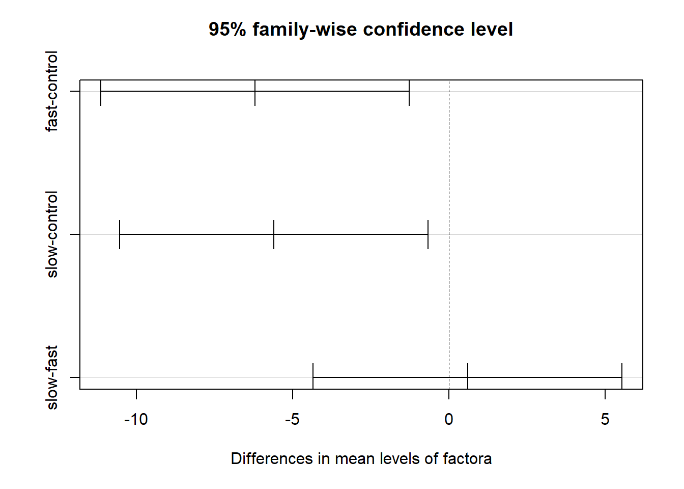
5.2 Using the asbio package for Post Hoc pairwise comparisons
Several functions in asbio are helpful for various multiple comparison tests. They each produce all possible pairwise group comparisons. The reader should utilize the help (e.g., ‘?lsdCI’) for documentation on these functions to see the array of options available.
First, the so-called Fisher’s Protected LSD test is obtained. Recall that when there are three groups, simulation work has shown that performing the LSD tests following a significant omnibus F test does afford protection from error rate inflation. But when the design has more than three groups, the LSD test CANNOT be recommended.
Several functions below can specify the model simply by passing the DV and IV a arguments, in that order.
# The asbio package has several functions that permit pairwise post hoc
# multiple comparison tests:
#require(asbio)
lsdCI(hays$dv,hays$factora)
##
## 95% LSD confidence intervals
##
## LSD Diff Lower Upper Decision Adj. p-value
## mucontrol-mufast 4.08691 6.2 2.11309 10.28691 Reject H0 0.00435
## mucontrol-muslow 4.08691 5.6 1.51309 9.68691 Reject H0 0.00907
## mufast-muslow 4.08691 -0.6 -4.68691 3.48691 FTR H0 0.76555Next is a simple bonferroni adjustment.
#require(asbio)
bonfCI(hays$dv,hays$factora)
##
## 95% Bonferroni confidence intervals
##
## Diff Lower Upper Decision Adj. p-value
## mucontrol-mufast 6.2 1.11592 11.28408 Reject H0 0.013052
## mucontrol-muslow 5.6 0.51592 10.68408 Reject H0 0.027217
## mufast-muslow -0.6 -5.68408 4.48408 FTR H0 1asbio also has a function for the standard Tukey test.
#require(asbio)
tukeyCI(hays$dv,hays$factora)
##
## 95% Tukey-Kramer confidence intervals
##
## Diff Lower Upper Decision Adj. p-value
## mucontrol-mufast 6.2 1.26141 11.13859 Reject H0 0.011723
## mucontrol-muslow 5.6 0.66141 10.53859 Reject H0 0.023855
## mufast-muslow -0.6 -5.53859 4.33859 FTR H0 0.951301Implementation of the Scheffe test is also possible
#require(asbio)
scheffeCI(hays$dv,hays$factora)
##
## 95% Scheffe confidence intervals
##
## Diff Lower Upper Decision Adj. P-value
## mucontrol-mufast 6.2 1.04108 11.35892 Reject H0 0.015929
## mucontrol-muslow 5.6 0.44108 10.75892 Reject H0 0.031227
## mufast-muslow -0.6 -5.75892 4.55892 FTR H0 0.955717In designs with a control group and several treatment conditions, a recommended approach is the use of the Dunnett test. This controls alpha-rate inflation for all pairwise comparisons involving the control condition vs each treatment.
# the asbio package permits implementation of the Dunnett test
# with specification of the ANOVA model and the level of the control group
#require(asbio)
dunnettCI(hays$dv,hays$factora,control="control")
##
## 95% Dunnett confidence intervals
##
## Diff Lower Upper Decision
## mufast-mucontrol -6.2 -10.848181 -1.551819 Reject H0
## muslow-mucontrol -5.6 -10.248181 -0.951819 Reject H05.3 Additional multiple comparison functions
An alternative function for performing the Dunnett test is found in multcomp. With any future work in R, you will see frequent use of the ghlt and mcp functions. One can simply pass the ‘aov’ fit object to the function. It is also possible to change the type of MC test to other “flavors” with the ‘linfct’ argument. See the help page on this function. ghlt is a very widely used function for multiple comparisons.
# The Dunnett test can also be obtained from the multcomp package.
#require(multcomp)
fit1.dunnett <- glht(fit.1,linfct=mcp(factora="Dunnett"))
# obtain CI's to test each difference
confint(fit1.dunnett, level = 0.95)
##
## Simultaneous Confidence Intervals
##
## Multiple Comparisons of Means: Dunnett Contrasts
##
##
## Fit: aov(formula = dv ~ factora, data = hays)
##
## Quantile = 2.3335
## 95% family-wise confidence level
##
##
## Linear Hypotheses:
## Estimate lwr upr
## fast - control == 0 -6.2000 -10.8480 -1.5520
## slow - control == 0 -5.6000 -10.2480 -0.9520The DTK package implements an alternative to the Tukey HSD method that permits application to data sets with unequal N’s and heterogenous variances. Notice that the CI’s are not the same for the base Tukey application and the DTK application owing to this capability for unequal N’s (which we don’t have) and heterogeneity.
#require(DTK)
# first, repeat the Tukey HSD test procedure in DTK to compare to above:
TK.test(hays$dv,hays$factora) # should give the same outcome as both to Tukey HSD approaches above
## Tukey multiple comparisons of means
## 95% family-wise confidence level
##
## Fit: aov(formula = x ~ f)
##
## $f
## diff lwr upr p adj
## fast-control -6.2 -11.138591 -1.2614086 0.0117228
## slow-control -5.6 -10.538591 -0.6614086 0.0238550
## slow-fast 0.6 -4.338591 5.5385914 0.9513012# now request the Dunnett-Tukey-Kramer test:
DTK.test(hays$dv,hays$factora)## [[1]]
## [1] 0.05
##
## [[2]]
## Diff Lower CI Upper CI
## fast-control -6.2 -12.634414 0.2344137
## slow-control -5.6 -10.629056 -0.5709442
## slow-fast 0.6 -4.507666 5.7076663The outcome with the Hays data set may be surprising. Note that, with ‘DTK’ the first comparison, fast vs ctl, has a CI that now overlaps zero, and is thus “NS”. The second comparison, slow vs ctl is a smaller mean difference, but the adjusted CI does not overlap zero. This differs from the standard Tukey HSD test.
Confusing? now look back at the descriptive statistics for these three groups. note that even though the homogeneity of variance tests were NS (a later section in this document), the std dev is smaller for the “slow” group. Since DTK does not use the pooled within group variance as the “error term” and uses Welch or Fisher-Behrens type error from just the two groups involved, the differences in the within-group variances can affect the outcome. The error df will also be smaller since the pooled MS is not used. Such discrepancies from “expected” outcomes can become even more extreme when n’s are unequal. This is a nice function to have available.
We can also plot the CI’s derived from DTK.
DTK.result <- DTK.test(hays$dv,hays$factora)
DTK.plot(DTK.result)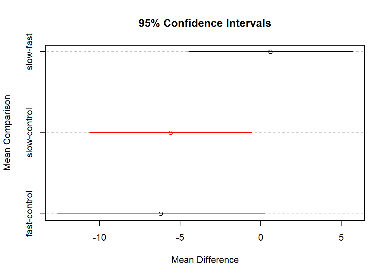
5.4 REGWQ is a recommended test
The mutoss package, provides an implementation of the Ryan / Einot and Gabriel / Welch test procedure (REGWQ). It is recognized as an acceptable improvement on the logic of the Newman Keuls procedure, a method which is not recommended. REGWQ typically requires equal N, but the package author has created a modification that permits unequal N using the Welch t test logic.
REGWQ is typically described as an approach using the studentized range statistic (as does Tukey HSD and Neuman Keuls), but the r-value for the q statistic is the average of the Tukey r and the N-K r. It is thought that it provides more power than N-K, while adequately controlling Type I error inflation (that N-K does not).
#require(mutoss)
#note: mutoss requires three packages not available on CRAN.  Obtain them from
# bioconductor. These packages are
# Biobase
# BioGenerics
# multtest
# to install, see
# http://www.bioconductor.org/packages/release/bioc/html/Biobase.html
# http://www.bioconductor.org/packages/release/bioc/html/BiocGenerics.html
# http://www.bioconductor.org/packages/release/bioc/html/multtest.html
regwq1 <- regwq(hays$dv~hays$factora, alpha=.05, data=hays)
## #----REGWQ - Ryan / Einot and Gabriel / Welsch test procedure
##
## Number of hyp.: 3
## Number of rej.: 2
## rejected pValues adjPValues
## 1 3 0.0091 0.0091
## 2 1 0.0117 0.0117regwq1## $adjPValues
## [1] "0.0117" "0.7655" "0.0091"
##
## $rejected
## [1] TRUE FALSE TRUE
##
## $statistic
## [1] 4.402 0.426 3.976
##
## $confIntervals
## [,1] [,2] [,3]
## control-fast 6.2 NA NA
## slow-fast 0.6 NA NA
## control-slow 5.6 NA NA
##
## $errorControl
## An object of class "ErrorControl"
## Slot "type":
## [1] "FWER"
##
## Slot "alpha":
## [1] 0.05
##
## Slot "k":
## numeric(0)
##
## Slot "q":
## numeric(0)5.5 The Games-Howell Modification of the Tukey Test
A commonly used post hoc test by psychology researchers is the games-howell modification of the tukey test for situations when unequal samples sizes and heterogeneity of variance are present.
5.5.1 The oneway function from userfriendlyscience has capabilities for post hoc tests.
The oneway function will provide the standard set of p.adjust capabilities for alpha rate adjustment (e.g., “holm”, “fdr”, “bonferroni”, etc). It will also implement the Tukey test and the Games-Howell modification of the Tukey test.
oneway(y=hays$dv, x=hays$factora, posthoc=c("tukey"))## ### Oneway Anova for y=dv and x=factora (groups: control, fast, slow)
##
## Omega squared: 95% CI = [.03; .5], point estimate = .25
## Eta Squared: 95% CI = [.06; .46], point estimate = .3
##
## SS Df MS F p
## Between groups (error + effect) 233.87 2 116.93 5.89 .008
## Within groups (error only) 535.6 27 19.84
##
##
## ### Post hoc test: tukey
##
## diff lwr upr p adj
## fast-control -6.2 -11.14 -1.26 .012
## slow-control -5.6 -10.54 -0.66 .024
## slow-fast 0.6 -4.34 5.54 .951oneway(y=hays$dv, x=hays$factora, posthoc=c("games-howell"))## ### Oneway Anova for y=dv and x=factora (groups: control, fast, slow)
##
## Omega squared: 95% CI = [.03; .5], point estimate = .25
## Eta Squared: 95% CI = [.06; .46], point estimate = .3
##
## SS Df MS F p
## Between groups (error + effect) 233.87 2 116.93 5.89 .008
## Within groups (error only) 535.6 27 19.84
##
##
## ### Post hoc test: games-howell
##
## diff ci.lo ci.hi t df p
## fast-control -6.2 -12.08 -0.32 2.69 17.99 .038
## slow-control -5.6 -10.35 -0.85 3.11 13.17 .021
## slow-fast 0.6 -4.23 5.43 0.33 13.03 .9435.5.2 A second way to implement the Games-Howell test.
I have found a script that does the test; I cannot vouch for the accuracy of this code - still testing it, but it does match what was produced by the oneway function above.
# http://aoki2.si.gunma-u.ac.jp/R/src/tukey.R
source("tukey_gh.R")
tukeygh(data=hays$dv,group=hays$factora,method="Games-Howell")
## $result1
## n Mean Variance
## Group1 10 27.4 26.04444
## Group2 10 21.2 27.06667
## Group3 10 21.8 6.40000
##
## $Games.Howell
## t df p
## 1:2 2.6902894 17.99333 0.03791342
## 1:3 3.1089795 13.17132 0.02087408
## 2:3 0.3279782 13.03080 0.94268531Aaron Schliegel has independently offered another function to perform the GH test, but I have not yet examined it and compared to the ones I use here.
5.6 Using the ‘pairwise.t.test’ function for MC tests
This section describes the very helpful ‘pairwise.t.test’ function. It has similarities to the logic we saw above with ‘p.adjust’. It has two major attractive features: 1. It permits use of many of the error-rate control methods in the “bonferroni” family that we have seen recommended. 2. It permits use of either the pooled within-group error term (when the HOV assumption is satisfied) or a Welch approach to the t statistic when heterogeneity of variance is present. This is the ‘pool.sd’ argument.
I list code for choosing may of the flavors of correction, but only show output for two.
# first, just do pairwise comparisons with bonferroni corrections
# assumes having done a set of three "contrasts".  should match results seen
# above in the BonferroniCI function from asbio.
pairwise.t.test(hays$dv,hays$factora,pool.sd=TRUE,p.adj="bonf")
##
## Pairwise comparisons using t tests with pooled SD
##
## data: hays$dv and hays$factora
##
## control fast
## fast 0.013 -
## slow 0.027 1.000
##
## P value adjustment method: bonferroni# We can change the approach to the Holm, Hochberg, Hommel,
# Benjamini and Hochberg, Benjamini&Yekutieli, and fdr corrections,
# as well as "none" which will give the same thing as the LSD test.
# Choice of these depends on several factors, including whether
# the contrasts examined are independent (and they are not since they
# are all of the pairwise comparisons,
# Of these modified bonferroni type of approaches, only the "BY"
# approach is probably the most appropriate here, since some of our
# comparisons are correlated and BY permits that correlation to be either
# positive or negative
#pairwise.t.test(dv,factora,pool.sd=TRUE,p.adj="holm")
#pairwise.t.test(dv,factora,pool.sd=TRUE,p.adj="hochberg")
#pairwise.t.test(dv,factora,pool.sd=TRUE,p.adj="hommel")
#pairwise.t.test(dv,factora,pool.sd=TRUE,p.adj="BH")
#pairwise.t.test(dv,factora,pool.sd=TRUE,p.adj="BY")
pairwise.t.test(hays$dv,hays$factora,pool.sd=TRUE,p.adj="fdr")##
## Pairwise comparisons using t tests with pooled SD
##
## data: hays$dv and hays$factora
##
## control fast
## fast 0.013 -
## slow 0.014 0.766
##
## P value adjustment method: fdr#pairwise.t.test(dv,factora,pool.sd=TRUE,p.adj="none")Now demonstrate two of these tests again, but use ‘pool.sd=FALSE’.
# note that setting pool.sd to FALSE changes the outcome since
# it employs a Welch or Fisher-Behrens type of approach
pairwise.t.test(hays$dv,hays$factora,pool.sd=FALSE,p.adj="bonf")
##
## Pairwise comparisons using t tests with non-pooled SD
##
## data: hays$dv and hays$factora
##
## control fast
## fast 0.045 -
## slow 0.025 1.000
##
## P value adjustment method: bonferroni# or
pairwise.t.test(hays$dv,hays$factora,pool.sd=FALSE,p.adj="fdr")##
## Pairwise comparisons using t tests with non-pooled SD
##
## data: hays$dv and hays$factora
##
## control fast
## fast 0.022 -
## slow 0.022 0.748
##
## P value adjustment method: fdrIt is interesting that contol vs fast is found to be significant here for the bonferroni test (p=.045). So simply using the non-pooled error is not sufficient to produce a NS test as was the case above for ‘DTK’. ‘DTK’ is more conservative because of the Tukey family derivation instead of the bonferroni family derivation.
5.7 The Neuman-keuls test
Psychology researchers had commonly used the Neuman-Keuls test for many decades, since it afforded a power improvement over the Tukey HSD test. Simulation work has now found that it underperforms in the core goal of controlling Type I error rate inflation. I cannot recommend it so I do not do an example here. However, if once is forced to use it (by misinformed advisors or collaborators), it is possible to find R functions to do it.
One possibility is the ‘SNK.test’ function in the agricolae package.
5.8 The glht function for post hoc tests and contrasts
The multcomp package has some capabilities for multiple comparisons that are useful for a variety of model objects, including aov and lm. If we apply glht here, requesting Tukey adjustments for pairwise comparisons, we find that it matches the output from the TukeyHSD function above (at least to three decimals). We use the fit.3lm object first produced with the lm function.
#library(multcomp)
glht.tukey <-glht(fit.3lm, linfct = mcp(factora="Tukey"))
summary(glht.tukey)
##
## Simultaneous Tests for General Linear Hypotheses
##
## Multiple Comparisons of Means: Tukey Contrasts
##
##
## Fit: lm(formula = dv ~ factora, data = hays)
##
## Linear Hypotheses:
## Estimate Std. Error t value Pr(>|t|)
## fast - control == 0 -6.200 1.992 -3.113 0.0117 *
## slow - control == 0 -5.600 1.992 -2.811 0.0239 *
## slow - fast == 0 0.600 1.992 0.301 0.9513
## ---
## Signif. codes: 0 '***' 0.001 '**' 0.01 '*' 0.05 '.' 0.1 ' ' 1
## (Adjusted p values reported -- single-step method)confint(glht.tukey)##
## Simultaneous Confidence Intervals
##
## Multiple Comparisons of Means: Tukey Contrasts
##
##
## Fit: lm(formula = dv ~ factora, data = hays)
##
## Quantile = 2.48
## 95% family-wise confidence level
##
##
## Linear Hypotheses:
## Estimate lwr upr
## fast - control == 0 -6.2000 -11.1398 -1.2602
## slow - control == 0 -5.6000 -10.5398 -0.6602
## slow - fast == 0 0.6000 -4.3398 5.5398The same glht function can also handle contrasts and they don’t have to be orthogonal. For example,
contr <- rbind("Ctl-Fast" = c(1, -1, 0),
               "Ctl-SLow" = c(1, 0, -1),
               "Fast-Slow"= c(0,1,-1))
glht.contr1 <-glht(fit.3lm,
                   linfct = mcp(factora=contr))
summary(glht.contr1, test=adjusted("holm"))
##
## Simultaneous Tests for General Linear Hypotheses
##
## Multiple Comparisons of Means: User-defined Contrasts
##
##
## Fit: lm(formula = dv ~ factora, data = hays)
##
## Linear Hypotheses:
## Estimate Std. Error t value Pr(>|t|)
## Ctl-Fast == 0 6.200 1.992 3.113 0.0131 *
## Ctl-SLow == 0 5.600 1.992 2.811 0.0181 *
## Fast-Slow == 0 -0.600 1.992 -0.301 0.7655
## ---
## Signif. codes: 0 '***' 0.001 '**' 0.01 '*' 0.05 '.' 0.1 ' ' 1
## (Adjusted p values reported -- holm method)summary(glht.contr1, test=adjusted("none"))##
## Simultaneous Tests for General Linear Hypotheses
##
## Multiple Comparisons of Means: User-defined Contrasts
##
##
## Fit: lm(formula = dv ~ factora, data = hays)
##
## Linear Hypotheses:
## Estimate Std. Error t value Pr(>|t|)
## Ctl-Fast == 0 6.200 1.992 3.113 0.00435 **
## Ctl-SLow == 0 5.600 1.992 2.811 0.00907 **
## Fast-Slow == 0 -0.600 1.992 -0.301 0.76555
## ---
## Signif. codes: 0 '***' 0.001 '**' 0.01 '*' 0.05 '.' 0.1 ' ' 1
## (Adjusted p values reported -- none method)confint(glht.contr1)##
## Simultaneous Confidence Intervals
##
## Multiple Comparisons of Means: User-defined Contrasts
##
##
## Fit: lm(formula = dv ~ factora, data = hays)
##
## Quantile = 2.4796
## 95% family-wise confidence level
##
##
## Linear Hypotheses:
## Estimate lwr upr
## Ctl-Fast == 0 6.2000 1.2611 11.1389
## Ctl-SLow == 0 5.6000 0.6611 10.5389
## Fast-Slow == 0 -0.6000 -5.5389 4.3389