Chapter 7 Assumptions: Evaluation and Methods for handling their violation
This section reviews both graphical and inferential methods for evaluating the assumptions for the 1-way ANOVA omnibus F test, and the use of the pooled within-group error for contrasts and multiple comparisions
7.1 Graphical evaluation of Residuals
In order to provide graphical displays for residuals analysis, R provides a very simple approach when working with linear models. All that is required is to request a plot of the model and this provides the relevant residuals plots. All four fits from above yield the same residuals, so lets just look at fit.2 since it used ‘lm’. This is the same approach we have covered for regresion models in R.
The first, commented, code line (‘plot(fit.2)’) produces all four plots and the user is required to click or hit the enter key to advance through the set. Instead, I request each individually, but only display the two we are most familiar with since they are the relevant ones here.
#win.graph()
#plot(fit.2)
# now produce the same 4 graphs in their own windows
plot(fit.2,which=1) #residuals vs yhats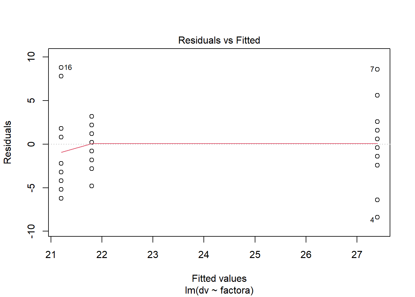
plot(fit.2,which=2) #normal probability plot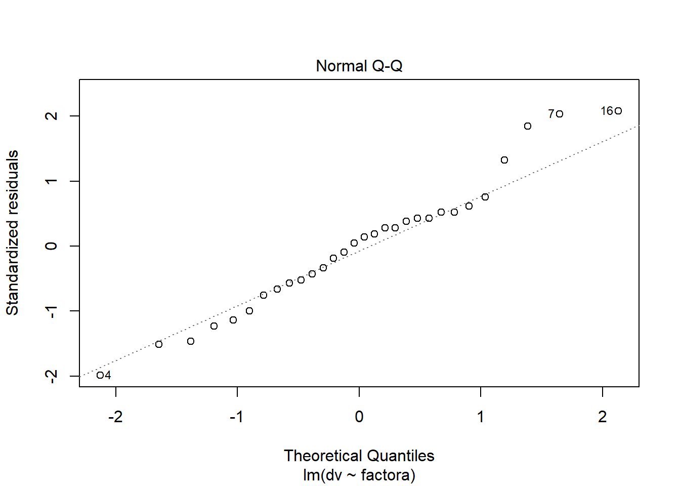
#plot(fit.2,which=3)
#plot(fit.2,which=5)
A better qq plot is available in the car package. It adds a confidence envelope to the qqnormal plot in order to better gauge, visually, how well the variable fits a normal distribution. Here, the residuals are extracted from the fit.2 lm object and passed to the qqPlot function.
car::qqPlot(fit.2$residuals, distribution="norm", id=FALSE)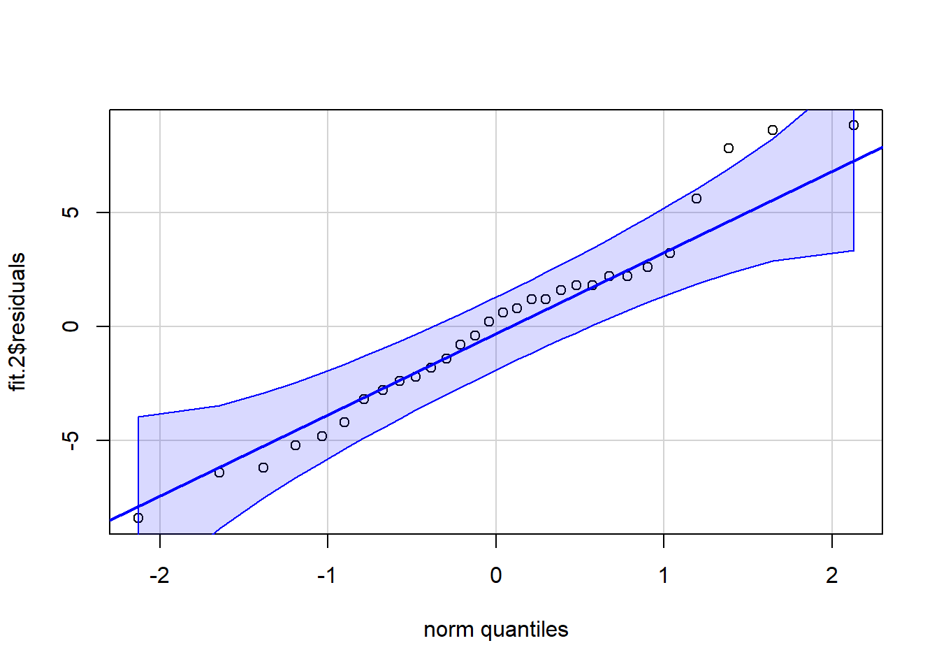
These standard plots produced by the base system ‘plot’ function do not include a frequency histogram of the residuals. It is useful, and can be done quickly by extracting the residuals from the ‘lm’ fit object and passing them directly to the ‘histogram’ function. In this illustration the histogram is not embellished with any additional text or style changes from defaults. The histogram would be more useful in larger N data sets than for this small example. In this example the deviation from normality is no too bad, especially for a small sample size study.
hist(fit.2$residuals, breaks=8, prob=TRUE)
lines(density(fit.2$residuals))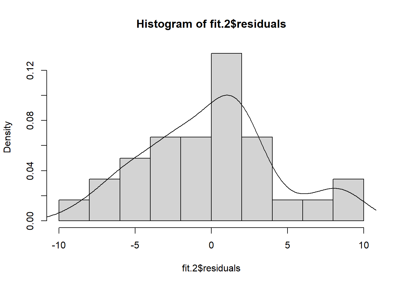
7.2 Inferences about the Normality Assumption
R provides several approaches to evaluation of the normality of a variable. The most well-known test is the Shapiro-Wilk test. That test is shown here along with the Anderson-Darling test which is (by my read) a preferred approach. Other tests are also available, and the code is shown, although commented out and not executed here. Note an alternative way of passing the ‘lm’ fit object residuals to a function rather than the ‘fit.2$residuals’ approach taken for the frequency histogram above. These tests do not permit rejection of the null hypothesis of residual normality, an outcome that is consistent with the visualizations done above.
# Perform the Shapiro-Wilk test for normality on the residuals
shapiro.test(residuals(fit.2))
##
## Shapiro-Wilk normality test
##
## data: residuals(fit.2)
## W = 0.97096, p-value = 0.5656# use tests found in the nortest package, as we reviewed for multiple regression
#library(nortest)
ad.test(residuals(fit.2)) #get Anderson-Darling test for normality (nortest package must be installed)##
## Anderson-Darling normality test
##
## data: residuals(fit.2)
## A = 0.30011, p-value = 0.5599#cvm.test(residuals(fit.2)) #get Cramer-von Mises test for normaility (nortest package must be installed)
#lillie.test(residuals(fit.2)) #get Lilliefors (Kolmogorov-Smirnov) test for normality (nortest package must be installed)
#pearson.test(residuals(fit.2)) #get Pearson chi-square test for normaility (nortest package must be installed)
#sf.test(residuals(fit.2)) #get Shapiro-Francia test for normaility (nortest package must be installed)7.3 Inferential tests regarding the homogeneity of Variance Assumption
Several tests are available in R for the ANOVA-related homogeneity of variance assumption. The reader will recall that we saw other tests of homoscedasticity for regression models in R code illustrations for those models. They are also appropriate here, but are not repeated in order to save space. The most common tests are those in the “Levene” family, but others are shown here as well.
The first test is The Bartlett Test from stats package (stats is part of the base install). This test is not identical to the Bartlett-Box test produced by SPSS MANOVA, but it is close. The Bartlett-Box F-test reported in MANOVA is an adaptation to the univariate case of the Box’s M test for multivariate data. The Bartlett test in R is based on an original paper by Bartlett (1937?) and should probably converge very closely on the Bartlett-Box F approximation. The Bartlett test statistic is a chi-squared approximation. This test is sensitive to departures from the normality in the DV.
bartlett.test(dv~factora,data=hays)##
## Bartlett test of homogeneity of variances
##
## data: dv by factora
## Bartlett's K-squared = 4.702, df = 2, p-value = 0.09527The Cochran’s C test for outlying variances is implemented in the outliers package. The function ‘cochran.test’ requires the model specification and the data frame for execution. The result appears to match the test result produced SPSS MANOVA for this same data set, but df are different. I have yet to explore the df question for each of these implementations. MANOVA reports 9,3 df where ‘cochran.test’ reports 10,3 df. The “sample estimates” are the variances of the individual cells.
cochran.test(dv~factora, hays)##
## Cochran test for outlying variance
##
## data: dv ~ factora
## C = 0.45482, df = 10, k = 3, p-value = 0.5093
## alternative hypothesis: Group fast has outlying variance
## sample estimates:
## control fast slow
## 26.04444 27.06667 6.40000We can find the Levene Test in the car package this is actually the Brown-Forsythe modification of the Levene test to be median-centered rather than mean-centered. We have seen that what some SPSS procedures call the Levene test is actually the original Levene test that uses mean-centering and is sensitive to the normality assumption. Here, the ‘leveneTest’ function has a default of median centering (the desireable approach)
#require(car)
leveneTest(dv~factora,data=hays)
## Levene's Test for Homogeneity of Variance (center = median)
## Df F value Pr(>F)
## group 2 2.0076 0.1539
## 27The Levene test can also be obtained from the lawstat package. The lawtstat version is more flexible, permitting mean centering,median centering, or trimmed-mean centering as well as bootstrapping.
First, let’s use the mean-centering approach and demonstrate that this is what SPSS uses in one-way and GLM (older versions of GLM).
#require(lawstat)
levene.test(hays$dv,hays$factora,location="mean")
##
## Classical Levene's test based on the absolute deviations from the mean
## ( none not applied because the location is not set to median )
##
## data: hays$dv
## Test Statistic = 2.0588, p-value = 0.1472Next is the median centering approach to match leveneTest from car, and to provide the Brown-Forsythe method that was the modification of Levene to be more robust against non-normality.
levene.test(hays$dv,hays$factora,location="median")##
## Modified robust Brown-Forsythe Levene-type test based on the absolute
## deviations from the median
##
## data: hays$dv
## Test Statistic = 2.0076, p-value = 0.1539A robust method used trimmed-mean centering; 20% of the scores are trimmed here.
levene.test(hays$dv,hays$factora,location="trim.mean",trim.alpha=.2)##
## Modified robust Levene-type test based on the absolute deviations from
## the trimmed mean ( none not applied because the location is not set to
## median )
##
## data: hays$dv
## Test Statistic = 2.0179, p-value = 0.1525This next approach returns to median centering, but implements the Obrien test which uses a correction factor described by Obrien (1978) and removal of zeros by Hines and Hines (2000). This is supposed to be a useful improvement on the basic Levene method and can be recommended.
levene.test(hays$dv,hays$factora,location="median", correction.method="zero.correction")##
## Modified robust Brown-Forsythe Levene-type test based on the absolute
## deviations from the median with modified structural zero removal method
## and correction factor
##
## data: hays$dv
## Test Statistic = 2.4397, p-value = 0.1085The ‘levene.test’ function from lawstat also permits a bootstrapping approach to obtaining a test of the HOV asumption using the basic Levene median centering approach. This is recommended if marked non-normality of the within-cell distributions exists.
#     uses the median-centered approach.  from Lim and Loh, 1996
levene.test(hays$dv,hays$factora,location="median",bootstrap=TRUE)
##
## bootstrap Modified robust Brown-Forsythe Levene-type test based on the
## absolute deviations from the median
##
## data: hays$dv
## Test Statistic = 2.0076, p-value = 0.152The Fligner-Killeen test is a method that produces a chi-squared test statistic for a homogeneity of variance test. The Fligner-Killen method is a non-parametric approach to the median-centering absolute value method. I’ve not read any literature comparing it’s efficacy to the suite of Levene-related methods. The user should do some homework on this method before employing it.
fligner.test(hays$dv~hays$factora,data=hays)##
## Fligner-Killeen test of homogeneity of variances
##
## data: hays$dv by hays$factora
## Fligner-Killeen:med chi-squared = 4.0696, df = 2, p-value = 0.1307Finally, as an instructional tool, we can build our own function to do the median-centered Levene Test. This gives the reader the details on what the test actually does. In addition, it exposes the reader to the ‘tapply’ function which is a very useful member of the “apply” family of functions. It permits us to do an operation (subtracting their group median from individual DV scores). These new absolute value deviations are then simply analyzed with a one-way anova (using ‘lm’ here). Note that the p-value matches what we obtained above for both ‘leveneTest’ and ‘levene.test’.
# Here,I build the Brown-Forsythe modification of the Levene test from scratch:
#  This should give you some insight into a bit of "The R Way"
bf.levene <- function(y, group)
   {
   group <- as.factor(group) # just to make certain the IV is a "factor"
   medians <- tapply(y, group, median)
   deviation <- abs(y - medians[group])
   anova(lm(deviation ~ group))
   }
bf.levene(hays$dv,hays$factora)
## Analysis of Variance Table
##
## Response: deviation
## Df Sum Sq Mean Sq F value Pr(>F)
## group 2 27.467 13.7333 2.0076 0.1539
## Residuals 27 184.700 6.84077.4 A plot of cell means vs variances
A caveat at the outset: this type of plot is not terribly useful for studies with only three groups. But with larger factorial anovas, it might be helpful.
We discussed this plot previously. Recall that this type of plot helps evaluate whether heterogeneity of variance might have arisen from a simple scaling issue. If so, then scale transformations may help. E.g,, a postive mean-variance correlation reflects a situation where a log transformation or a fractional exponent transformation of the DV might produce homoscedasticity. I’m also using the tapply function here in ways that we have not covered. tapply is an important function in dealing with factors.
The issue with this particular design/plot is that a scatterplot with only three points cannot possibly be relied upon to reveal a pattern. Nonetheless, it puts in place a technique for future use in other design.
plot(tapply(hays$dv, hays$factora, mean), tapply(hays$dv, hays$factora, var), xlab = "Cell Means",
             ylab = "Cell Variances", pch = levels(hays$factora))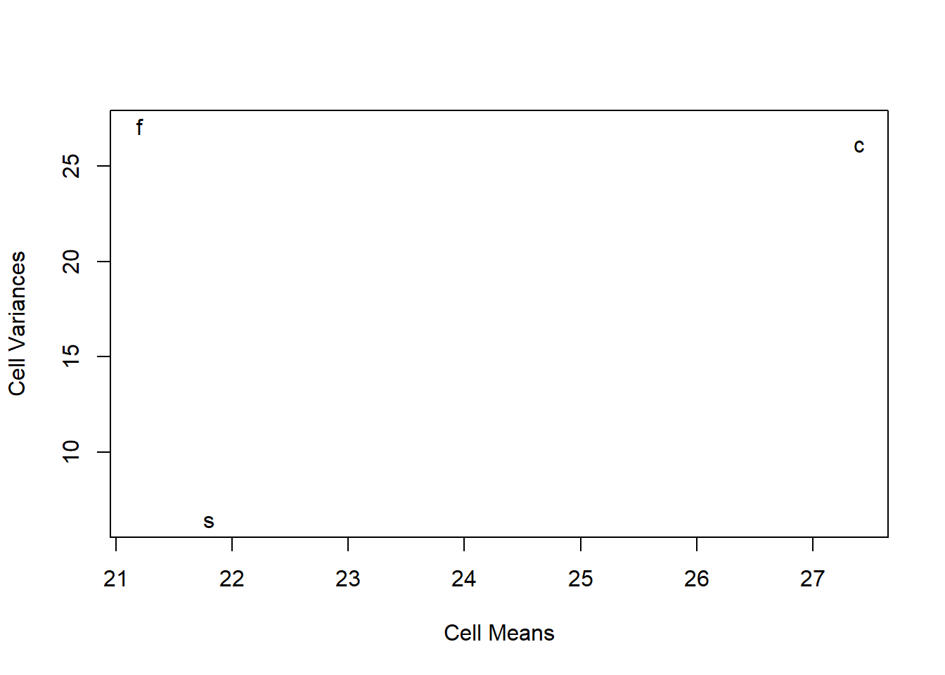
7.5 What to do when assumptions are violated
Useful strategies are available for addressing inferential questions from a 1-factor ANOVA design when assumptions are violated. Their number is very large. Some will be listed here. What is important for the student is to realize that alternatives to both the omnibus F-test and followup questions (e.g. contrasts, post hoc and other multiple comparison methods) are available.
Alternatives to the standard Omnibus F-test:
- Welch F test when Heterogeneity of Variance is present. This test was illustrated above with the ‘oneway.test’ funciton.
- A Brown-Forsythe modification of the F test is analogous to the Welch F test and is found in output from the
onewayfunction earlier in this document. - Bootstrapping or permutation tests when non-normality is present A permutation test was seen above with the ‘exAnova’ function. Bootstrapping is also availble in R and can be applied to ANOVA models. These Resampling methods are covered briefly in a later chapter
- Robust methods based on robust central tendency estimators (see the WRS2 package in R and much work by Rand Wilcox - and a later chapter in this document)
- Nonparametric methods are often used when DV distributions are divergent from normality. One of those is covered below, the Kruskall-Wallis test.
Alternatives to Post Hoc and Multiple Comparison Tests:
- Several MC tests are explicitly designed to cope with distributional assumption issues in ANOVA data sets. These are discussed below in the Post Hoc/MC section
- One very commonly used approach in the psychological sciences is the “Games-Howell” modification of the Tukey test for situations with Heterogeneity of Variance and Unequal N. Other more recent approaches may be an improvement on the G-H method, but have not received as much usage since they had only recently become available in software.
- The DTK test (Duncan/Tukey/Kramer) is another modification of the Tukey HSD test for applications when there is unequal N and heterogeneity of variance. See the Post Hoc / Multiple Comparisons section below.
- The Kruskall-Wallis test can also be followed up with nonparametric approaches to pairwise multiple comparisons (see below)
Alternatives for Analytical Contrasts when assumptions are violated:
- Most commonly, when heterogeneity of variance is present, the approach to follow up analysis involves one of the pairwise multiple comparison methods designed to cope with that heterogeneity (see below).
- However, since any analytical contrast is viewed as a linear combination, standard errors can be derived in the same manner as the Welch omnibus test is designed. I am still looking for a simple implementation of this in R with regard to ANOVA contrasts. The emmeans package provides one possible solution and was introduced above I am still sorting out some confusions about use of emmeans for these purposes.