Chapter 4 Alternatives to aov and lm for 1-way ANOVA
Several add-on packages provide alternate approaches to doing ANOVAs. Both ez and afex are broadly capable and attempt to simplify some of the techniques to doing the various components of analyzing different designs. A choice among them, vs using aov and/or lm is largely a matter of style and preference but each adds components that may be desired. The granova functions are useful for exploring some of the theoretical components of ANOVA, using unique graphical approaches. They are probably most helpful as instructional tools, and the 1-way design illustration here is an example of that.
4.1 The oneway function from the userfriendlyscience package
The userfriendlyscience package has a group of functions that are intended to ease the transition of researchers from use of SPSS to R. It contains a flexible function named oneway for implementation of 1-way ANOVA.
A potentially nice graph that shows data points and violin plots for each group can also be provided, but unfortunately it creates a line graph. Corrections for heterogeneity of variance are also provided.
The function has a capability of implementing the Levene test, but since it is the mean-centered version, that argument is not included here. Arguments for returning means and other descriptive statistics are present but not included here since, as of this writing, it produces an error in how the psych::describeBy function is implemented.
In a later chapter, we will see how to obtain post hoc tests by using a “posthoc” argument.
oneway(y=hays$dv, x=hays$factora, plot=TRUE, corrections=TRUE)## ### Oneway Anova for y=dv and x=factora (groups: control, fast, slow)## Registered S3 methods overwritten by 'ufs':
## method from
## grid.draw.ggProportionPlot userfriendlyscience
## pander.associationMatrix userfriendlyscience
## pander.dataShape userfriendlyscience
## pander.descr userfriendlyscience
## pander.normalityAssessment userfriendlyscience
## print.CramersV userfriendlyscience
## print.associationMatrix userfriendlyscience
## print.confIntOmegaSq userfriendlyscience
## print.confIntV userfriendlyscience
## print.dataShape userfriendlyscience
## print.descr userfriendlyscience
## print.ggProportionPlot userfriendlyscience
## print.meanConfInt userfriendlyscience
## print.multiVarFreq userfriendlyscience
## print.normalityAssessment userfriendlyscience
## print.regrInfluential userfriendlyscience
## print.scaleDiagnosis userfriendlyscience
## print.scaleStructure userfriendlyscience
## print.scatterMatrix userfriendlyscience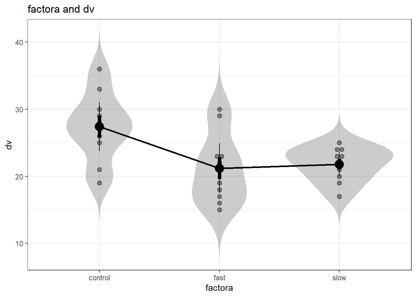
## Omega squared: 95% CI = [.03; .5], point estimate = .25
## Eta Squared: 95% CI = [.06; .46], point estimate = .3
##
##                                     SS Df     MS    F    p
## Between groups (error + effect) 233.87  2 116.93 5.89 .008
## Within groups (error only)       535.6 27  19.84
##
##
## ### Welch correction for nonhomogeneous variances:
##
## F[2, 15.91] = 5.07, p = .02.
##
## ### Brown-Forsythe correction for nonhomogeneous variances:
##
## F[2, 21.95] = 5.89, p = .009.
4.2 Using the granova package
The *granova package provides a unique approach to the oneway ANOVA design. It includes a rather neat graph that summarizes the ANOVA components. BEWARE, the “contrast coefficients” are not the analytical contrast types of coefficients we have been working with. Instead, we would call these treatment deviation contrasts - deviations of each cell mean from the grand mean. These are thus the regression coefficient values that emerge from effect coding.
The granova.1w function produces both a standard numeric output and a figure. The components of the figure are described in class, but it is simple to find the grand mean, the cell means and the data on the plot.
One caution about implementing granova.1w:
granova.1w can take either a data frame as the first argument, or the DV and IV variable names as the first two arguments. If we were passing the data frame as the first argument, the data frame must meet exact specifications. Only DV values can be included and the different columns must be the different groups - equal sample sizes required. This is a bit of a clunky method so we will use the second method. We execute the code by passing the DV and IV names.
When the numerator and denominator MS for the F test are depicted as “squares”, it becomes clear that the F ratio is the ratio of the area of MSbetween to MSwithin. The X axis is scaled as the deviation quantity for each cell mean relative to the grand mean; therefore the X axis has a mean of zero. Unfortunately for the color blind, the red triangles for cell means/deviations and the green circle for the grand mean may not be distinguishable via color but the shapes are distinct.
#require(granova)
kable(granova.1w(hays$dv, hays$factora,res=TRUE))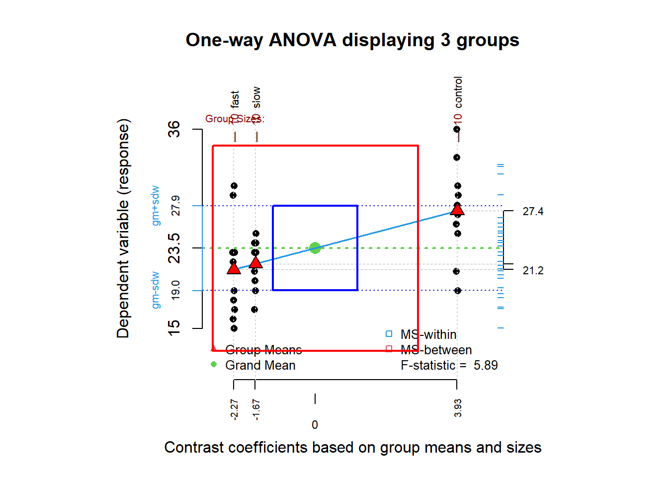
|
|
Granova also permits use of predefined, a priori, contrasts of the style we have used so heavily, with the granova.contr function. If we define the same orthogonal set used above (for fit.3 and fit.4), then the granova.contr function generates some nice plots along with the tests of the contrasts, and a standardized effect size estimate for each contrast. Very Nice. BUT BE CAREFUL……‘granova.contr’ needs to have equal N, and a data frame sorted on the factor (the grouping variable, in the order implied by the contrast coefficients.
contrasts.factora <- matrix(c(2,-1,-1, 0,1,-1),ncol=2)
granova.contr(hays$dv,contrasts.factora)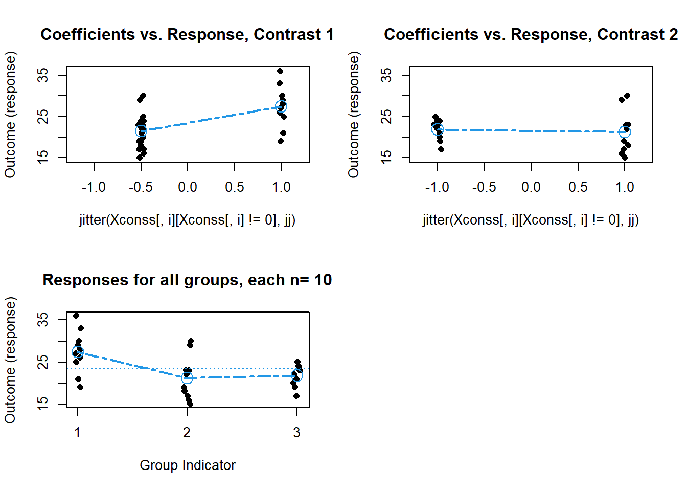
## $summary.lm
##
## Call:
## lm(formula = resp ~ contrst)
##
## Residuals:
##    Min     1Q Median     3Q    Max
##   -8.4   -2.7    0.4    2.1    8.8
##
## Coefficients:
##             Estimate Std. Error t value Pr(>|t|)
## (Intercept)  23.4667     0.8132  28.858   <2e-16 ***
## contrst1      3.9333     1.1500   3.420    0.002 **
## contrst2     -0.3000     0.9959  -0.301    0.766
## ---
## Signif. codes:  0 '***' 0.001 '**' 0.01 '*' 0.05 '.' 0.1 ' ' 1
##
## Residual standard error: 4.454 on 27 degrees of freedom
## Multiple R-squared:  0.3039, Adjusted R-squared:  0.2524
## F-statistic: 5.895 on 2 and 27 DF,  p-value: 0.007513
##
##
## $means.pos.neg.coeff
##    neg  pos diff stEftSze
## 1 21.5 27.4  5.9     1.32
## 2 21.8 21.2 -0.6    -0.13
##
## $contrasts
##      [,1] [,2]
## [1,]  1.0    0
## [2,] -0.5    1
## [3,] -0.5   -1
##
## $group.means.sds
##       [,1] [,2]  [,3]
## Means 27.4 21.2 21.80
## S.D.s  5.1  5.2  2.53
##
## $data
##       [,1] [,2] [,3]
##  [1,]   27   23   23
##  [2,]   28   22   24
##  [3,]   33   18   21
##  [4,]   19   15   25
##  [5,]   25   29   19
##  [6,]   29   30   24
##  [7,]   36   23   22
##  [8,]   30   16   17
##  [9,]   26   19   20
## [10,]   21   17   23
Conclusion:
Granova is a fascinating approach. It gives all of the basics we need. The graphs that are produced are very helpful in an instructional context, reminding us what “Mean Squares” means. But I have never seen this plot used for a research publication. One would likely have to spend a large amount of time convincing an editor and reviewers of its value.
The recommendation here is to use it as a sort of exploratory device rather than for the production of a publication quality graph.
4.3 Use of the ez package
Among a number of additional ways to obtain ANOVA results for experimental designs, the ez package intends to be comprehensive ANOVA modeling suite. It requires a unique way of specifying the DV, IV, and several other components. Once the syntax is learned, many R users have found it to be efficient. I find that it adds nothing to what we have accomplished above for 1-way designs, but it may be useful for factorial designs.
The EZ package contains the ezAnova function which serves as a wrapper for many of the things shown above. It is a quick way to obtain a fairly full analysis. It does not appear to enable inferences regarding analytical/orthogonal contrasts. emmeans would have to be used as a supplement in order to obtain them.
Note at the outset that functions from ez require a data frame that contains a case number (subject number) variable. Since the original hays data frame was sorted by group, it made it easy to simply specify subject (case) number as the sequential order number of the case in the data frame. Since the ez ANOVA functions permit an argument that specifies the data frame, we don’t have to be concerned about conflicts arising because the original hays data frame was “attached”.
#require(ez)
# in order to use ez functions we need a subject number variable in the data frame
snum <- ordered(rownames(hays))
hays2 <- cbind(snum,hays)
# examine hays2
headTail(hays2)
## snum factora dv
## 1 1 control 27
## 2 2 control 28
## 3 3 control 33
## 4 4 control 19
## ... <NA> <NA> ...
## 27 27 slow 22
## 28 28 slow 17
## 29 29 slow 20
## 30 30 slow 23# first, obtain descriptives; note that FLSD is Fisher's LSD critical value
# note that Fisher's Least Significant Difference is computed as
# sqrt(2)*qt(.975,DFd)*sqrt(MSd/N), where N is taken as the mean N
# per group in cases of unbalanced designs.
descript1 <- ezStats(
data = hays2,
dv = .(dv),
wid= .(snum),
between= .(factora))## Coefficient covariances computed by hccm()print(descript1)## factora N Mean SD FLSD
## 1 control 10 27.4 5.103376 4.086908
## 2 fast 10 21.2 5.202563 4.086908
## 3 slow 10 21.8 2.529822 4.086908The ezPlot function provides graphing capabilities tailored to the experimental design. I found it interesting that the error bars on the figure are derived from a generalized standard error of the mean based on the MSerror from the ANOVA, rather than the individual standard errors for each group, which are not actually used for anything.
# now plot the cell means and error bars.
# error bars based on GSEM as described above for Fishers LSD
plot1 <- ezPlot(
           data = hays2,
           dv = .(dv),
           wid= .(snum),
           between= .(factora),
           x = .(factora),
           do_lines=FALSE, do_bars=TRUE,
           x_lab= 'Treatment Group',
           y_lab= 'Mean DV Score')
## Coefficient covariances computed by hccm()print(plot1)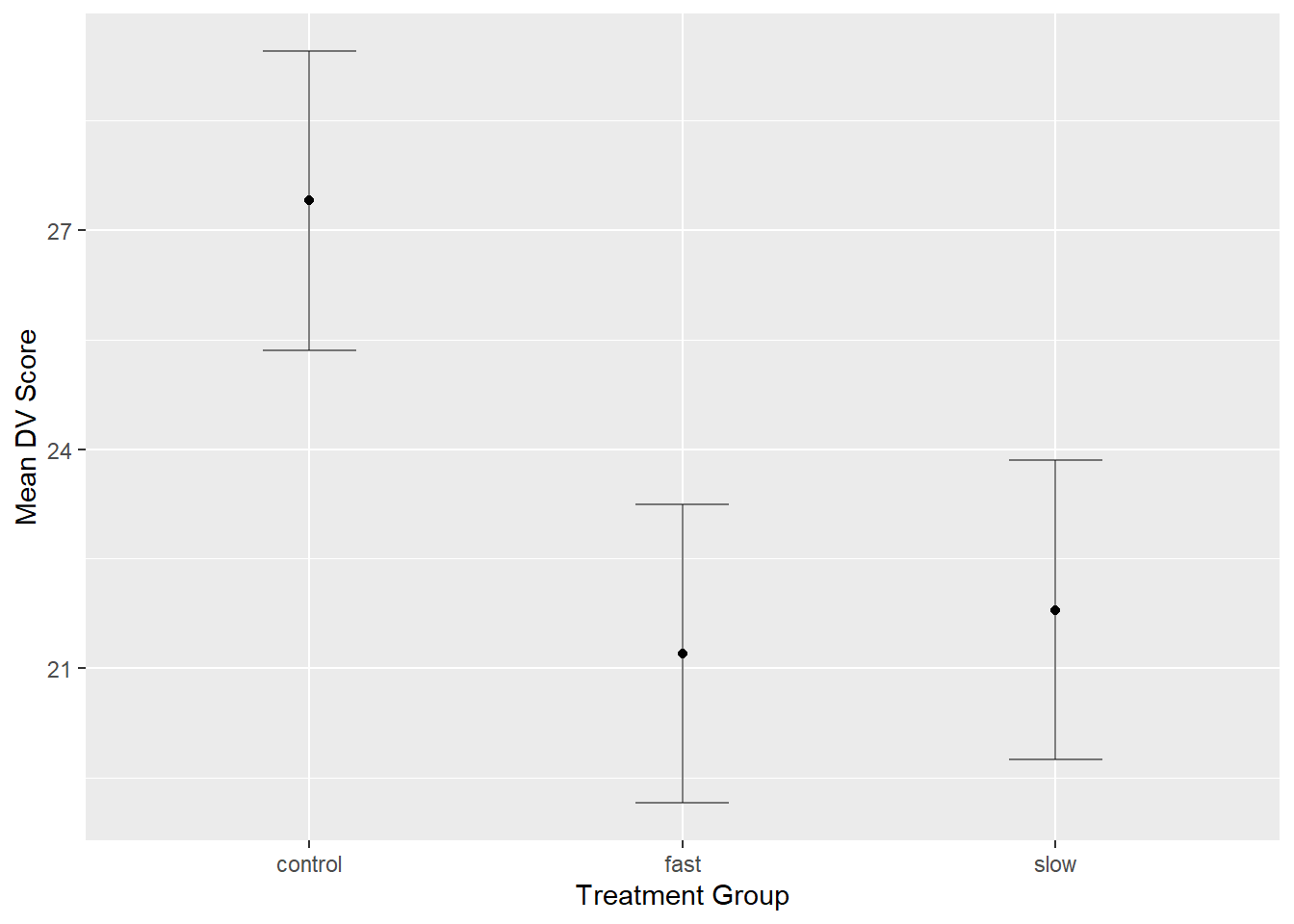
Use of the ezANOVA function involves a novel style of code, using a non-intuitive dot notation for specifying IVs, but one becomes accustomed to this fairly quickly. Once again, the same values for SS/F/pvalue are produced. An added benefit is that the Levene homogeneity of variance test is automatically generated (the median-centered version). It is important that an effect size indicator is also provided (“ges”, discussed elsewhere - or read the help page on the ez package).
# now do the 1way ANOVA
fit.4ez <- ezANOVA(
           data = hays2,
           dv = .(dv),
           between= .(factora),
           wid=snum,
           detailed=TRUE)
## Coefficient covariances computed by hccm()print(fit.4ez)## $ANOVA
## Effect DFn DFd SSn SSd F p p<.05 ges
## 1 factora 2 27 233.8667 535.6 5.894698 0.007512513 * 0.3039335
##
## $`Levene's Test for Homogeneity of Variance`
## DFn DFd SSn SSd F p p<.05
## 1 2 27 27.46667 184.7 2.00758 0.1538727By default, ezANOVA employs Type II SS decompositions. Although this distinction is only relevant for factorial designs (and unequal sample sizes) it would be useful to put in place the argument that permits specification of other SS types. The following code requests Type III SS. Unfortunately the output does not label the SS Type, so one has to be certain with the code.
# now do the 1way ANOVA
fit.4bez <- ezANOVA(
           data = hays2,
           dv = dv,
           between= .(factora),
           wid=snum,
           type=3,
           detailed=TRUE)
## Coefficient covariances computed by hccm()print(fit.4bez)## $ANOVA
## Effect DFn DFd SSn SSd F p p<.05 ges
## 1 (Intercept) 1 27 16520.5333 535.6 832.812547 7.900265e-22 * 0.9685978
## 2 factora 2 27 233.8667 535.6 5.894698 7.512513e-03 * 0.3039335
##
## $`Levene's Test for Homogeneity of Variance`
## DFn DFd SSn SSd F p p<.05
## 1 2 27 27.46667 184.7 2.00758 0.1538727EZ permits resampling tests. Here, we implement a permutation test. I show the code but suppress a lengthy status printout while it is doing the resampling. The result of the test is obtained in the next code chunk. The permutation algorithm is fairly slow and I don’t know if the ezPerm function can address analytical contrasts. We will revist permutation tests in a later chapter.
# now do the 1way anova as a permutation test
fit.5ezperm <- ezPerm(
           data = hays2,
           dv = dv,
           between= .(factora),
           snum,
perm= 1e3)fit.5ezperm## Effect p p<.05
## 1 factora 0.006 *The ez packages has functions to perfom bootstrapping, but right now older code that I used is broken and I’ve not yet sorted out why, so bootstrapping excluded for now. We can return to bootstrapping in a later chapter.
One additional capability in ez is an interesting graphical approach to displaying the data set. T This plot is Not the values of the DV, but locations where the various groups of cases are in the ordering of the data frame.
# other useful functions in the ez package
#win.graph()
ezDesign(
           data = hays2,
           x= .(factora),
           y= .(snum),
           row=NULL,col=NULL,
           cell_border_size=8)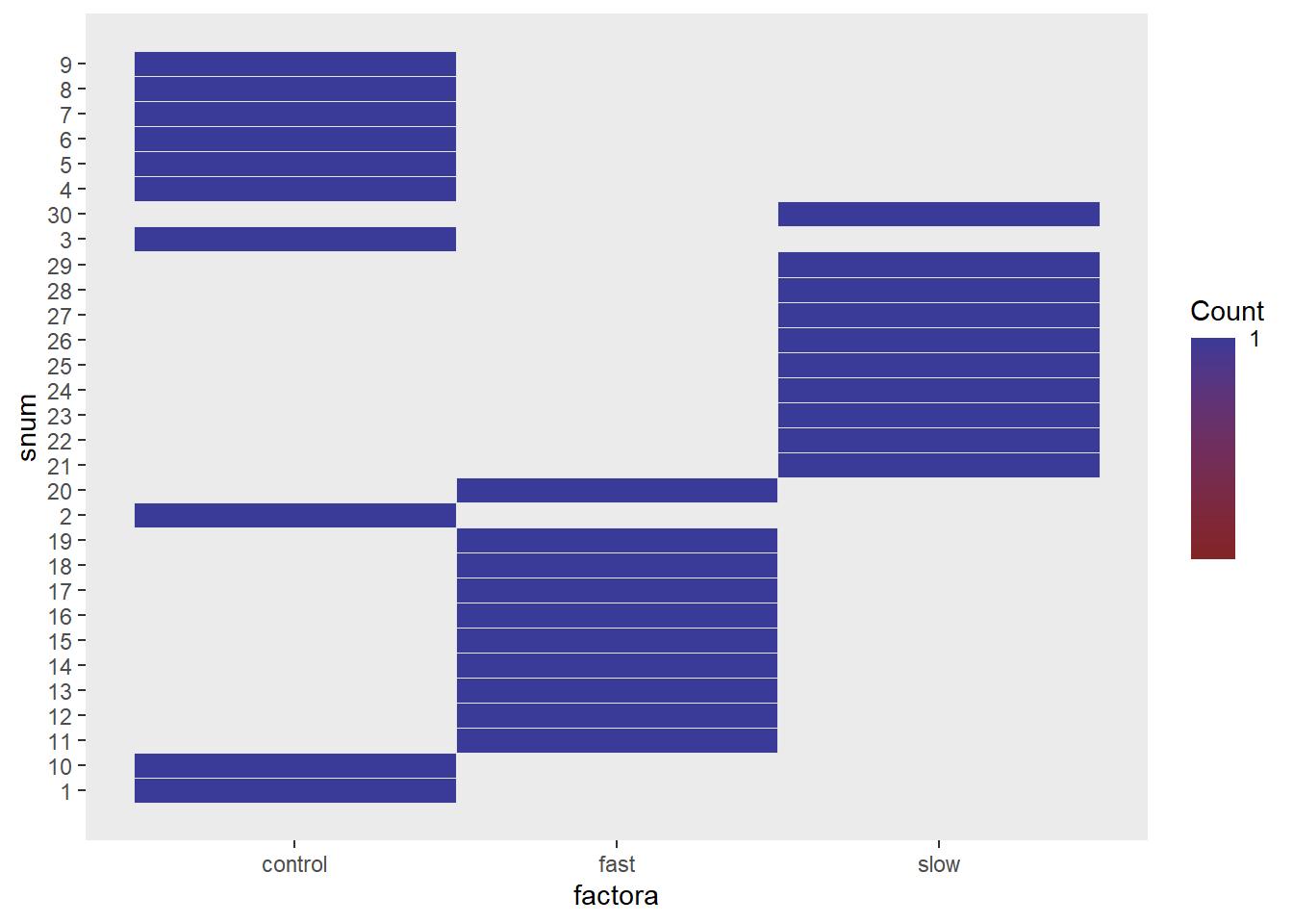
4.4 Using the afex package
The afex package is a wrapper for lm, car, and lme4 functions, the latter to do mixed models. The stated goals are a comprehensive set of functions for virtually all kinds of ANOVA models. My initial investigations into its usage have engendered a mix of optimism and concern over the scope of what it can do, the kinds of decisions that were made about restricting some kinds of ANOVA approaches, and ease of use. What is presented here is the bare bones analysis of our 3 group design. This section may expand as I become more skilled with afex.
First, lets use the “car” flavor of the afex approach to model the 3-group data set. Note that afex requires a data frame that has an identifier variables (such as subject number). I created such a data frame for the ez package functions above, so we can use the same “hays2” data frame here as well. Note that even though we have “attached” the original hays data frame, there is no conflict that arises by using the same variable names in hays2. This is because the afex functions permit naming the data frame as an argument.
In using afex, we choose one of three styles of specifying the model. The first shown here models on how the specification would be made in doing ANOVAs using functions from the car package. The afex package functon is thus aov_car. Unlike what we have seen above, this approach requires specification of the error factor - the “snum” variable is the case identifier and serves this role. We can think of the error as the variation in the DV due to snum within the factora levels.
Note that the aov_car function changes factor coding to what we have called “effect” coding (also known as deviation coding). In R, this is defined as contr.sum.
# needs data frame with subj id. use hays2.csv
fitx1 <- aov_car(dv~factora + Error(snum), data=hays2)
## Contrasts set to contr.sum for the following variables: factorafitx1## Anova Table (Type 3 tests)
##
## Response: dv
## Effect df MSE F ges p.value
## 1 factora 2, 27 19.84 5.89 ** .304 .008
## ---
## Signif. codes: 0 '***' 0.001 '**' 0.01 '*' 0.05 '+' 0.1 ' ' 1A bit better layout and info provision is possible with the ‘return’ argument, although we lose the “ges” effect size indicator.
# obtain a fuller table but without the effect size
fitx2 <- aov_car(dv~factora + Error(snum), data=hays2, return="univariate" )
## Contrasts set to contr.sum for the following variables: factorafitx2## Anova Table (Type III tests)
##
## Response: dv
## Sum Sq Df F value Pr(>F)
## (Intercept) 16520.5 1 832.8125 < 2.2e-16 ***
## factora 233.9 2 5.8947 0.007513 **
## Residuals 535.6 27
## ---
## Signif. codes: 0 '***' 0.001 '**' 0.01 '*' 0.05 '.' 0.1 ' ' 1Notice that with aov_car, the SS decomposition is, by default, Type III. Adding a “type” argument permits control of this characteristic. But in our 1way design with equal N, there is no difference in Type I, II, and III SS. The illustration is done here as a placeholder for what we will do later with factorial designs.
# obtain a fuller table but without the effect size
fitx2b <- aov_car(dv~factora + Error(snum), data=hays2, return="univariate", type=2)
## Contrasts set to contr.sum for the following variables: factorafitx2b## Anova Table (Type II tests)
##
## Response: dv
## Sum Sq Df F value Pr(>F)
## factora 233.87 2 5.8947 0.007513 **
## Residuals 535.60 27
## ---
## Signif. codes: 0 '***' 0.001 '**' 0.01 '*' 0.05 '.' 0.1 ' ' 1Postscript on current status of afex usage here:
Some advantages of using afex for other designs will be seen in later work with factorial and repeated measures designs. However, for our one-way anova needs here, this package adds only one thing. That is the “generalized effect size” (called ges) obtained with fitx1. In a oneway model, the ges is identical to the eta squared. The basic ANOVA with SS, df, F’s and pvalue are obviously the same as we have derived many other ways earlier in this document.
In conjunction with ‘glht’ and emmeans, afex has some broadly capable methods for implementing analytical contrasts and post hoc testing methods. Some of those illustrations are found in succeeding chapters.