Chapter 15 Bayes Factor approach to multiple regression

There are many approaches and flavors of Bayesian inference. A major set of tools is found in the Stan libraries. In R, these are implemented in the rstan package. There are extensive ways of doing inference for linear models (and many other models) using rstan tools. These approaches are often laborious, and require far more background in Bayesian methods than most readers of this document will have at this point in time. An alternative approach involves BUGS algorithms. They are implemented in WinBugs for the Windows platform and OpenBugs. An R package wwritten by Andrew Gelman is an interface to WinBugs or OpenBugs and is called R2WinBUGS. These packages are not illustrated here, but links to useful sites are:

[https://mc-stan.org/users/interfaces/rstan]

[https://cran.r-project.org/web/packages/R2WinBUGS/index.html]

In recent years, another kind of bayesian inference has gained traction is social, behavioral, and life sciences. This approach involves a focus on Bayes Factors as an index of support for or against hypotheses. It is not the purpose of this document to provide a full background on the Bayes Factor logic or method. Nonetheless, it is fairly simple to implement a Bayes Factor analysis of the rudimentary multiple regression methods covered in this document.

15.1 Basic approaches with Bayes Factors

The BayesFactor package, developed by Richard Morey (Morey & Rouder, 2018), is well documented and extensive tutorials are available.

For example:

[https://richarddmorey.github.io/BayesFactor/]

This section provides a brief overview of rudimentary analyses that create Bayes Factor evaluations of the linear model. I will use the two-IV model that we settled on as a reasonable one, the one with degrees_yr and cits as IVs and salary as DV. First, the ordinary least squares model is repeated so that we can compare results.

olsfit <- lm(salary~degree_yrs+cits,data=cohen1)
kable(tidy(olsfit))

term	estimate	std.error	statistic	p.value
(Intercept)	39073.6747	2396.47360	16.304655	0.0000000
degree_yrs	1061.7642	227.17563	4.673759	0.0000176
cits	212.1116	56.59392	3.747958	0.0004078

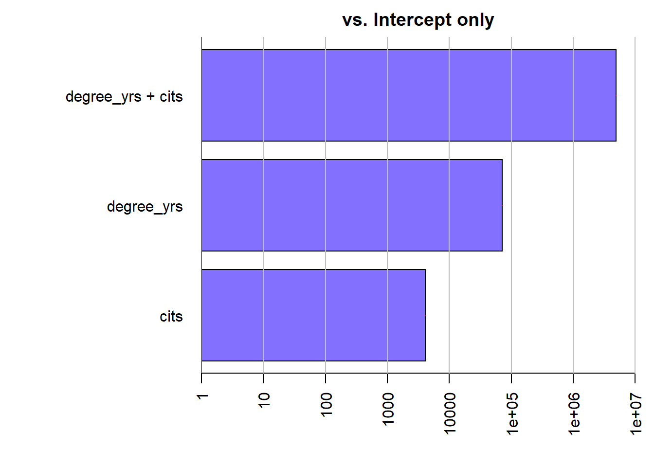
The regressionBF function permits simultaneous comparison of several models. Evaluation of only one model can use the lmBF function. The goal is the calculation of Bayes Factor indices permitting comparison of models and yeilding a metric that is interpreted as relative evidence for one hypothesis over another. Initially here, the regressionBF function is used to assess three different models against an “intercept-only” model. And then we will compare the three models against each other. Why three models? With two IVs there are three possible models of interest - one each with a single IV and a third with both IVs With the large sample size and the sizeable correlations of degree_yrs and cits with salary, it is not surprising that each model yields a Bayes Factor that is a very large value. The BF is interpreted as a ratio. For example, the degree_yrs - only model is found to be over 7000 times more likely than the intercept-only model. The two-IV model has extremely an extremely large BF. It is important to understand that there is substantial theory underlying the BF computation and assumptions have been made to create default shape and scaling of choices for the prior. The reader is expected to become skilled in these choices and the theory before use of these methods.

bf1 <- regressionBF(salary~degree_yrs+cits, data=cohen1)
bf1

## Bayes factor analysis
## --------------
## [1] degree_yrs        : 71125.54 ±0.01%
## [2] cits              : 4126.233 ±0%
## [3] degree_yrs + cits : 4963640  ±0%
## 
## Against denominator:
##   Intercept only 
## ---
## Bayes factor type: BFlinearModel, JZS

At this point we have seen that both the OLS and BF models offer strong support for the idea that the degree_yrs plus cits model is a strong one. But it might be informative to look at a model that has much weaker evidence.

We can reconsider the model that used gender as an IV. It was not a signficant predictor in the OLS model, which is repeated here.

olsfit2 <- lm(salary~gender,data=cohen1)
kable(tidy(olsfit2))

term	estimate	std.error	statistic	p.value
(Intercept)	52650.000	1810.539	29.079734	0.0000000
gendermale	3949.324	2444.918	1.615319	0.1114884

In a BayesFactor analysis we find a very different sized BF than for the degree_yrs+cits model. A BF value of 1.0 would indicate equivalent support for the null hypothesis (\(\beta\)=0) and the alternative (\(\beta \ne 0\)). The BF value found here (.773) indicates equivocal support for each with only very slight evidence favoring the null. We can take the reciprocal of the BF to find the degree of relative evidence for the null. That value is 1/.773 or 1.29. So we would say that the null is 1.29 times more likely than the null

bf1b <- lmBF(salary~gender, data=cohen1)
bf1b

## Bayes factor analysis
## --------------
## [1] gender : 0.7726611 ±0.01%
## 
## Against denominator:
##   Intercept only 
## ---
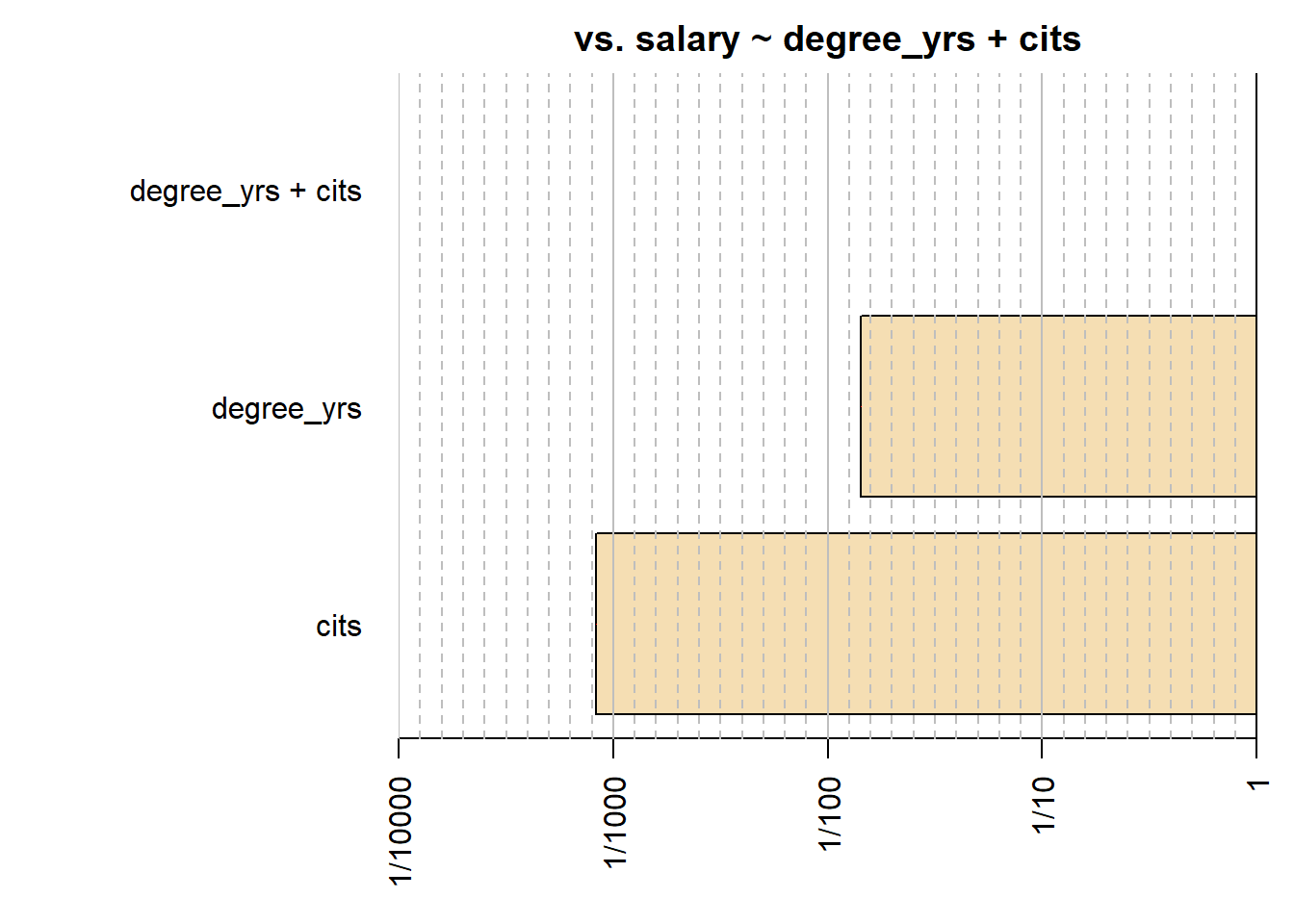
## Bayes factor type: BFlinearModel, JZS

Returning to the original two-IV model, the BayesFactor package permits some interesting and useful approaches to model comparison. Above, we only compared each of the three possible models to an intercept-only model. Now, we will compare them to each other. The relative evidence for one particular model can be found by taking the ratio of the BF to those models. Here, I compare the “best” model (using max) to each of the others. First, see that comparing the best model (the two-IV model) to itself yields a ratio of 1, and this makes sense. Against the twomodel,degree_yrs-only has less than 2% the strength of evidence times the strength of evidence. Or take the reciprocal and find that the two-IV model is nearly 70 times more likely Against the cits-only model the two-IV model fares even better with the cits-only model garnering less than .1% support.

bf2 <- bf1/max(bf1)
bf2

## Bayes factor analysis
## --------------
## [1] degree_yrs        : 0.01432931   ±0.01%
## [2] cits              : 0.0008312918 ±0%
## [3] degree_yrs + cits : 1            ±0%
## 
## Against denominator:
##   salary ~ degree_yrs + cits 
## ---
## Bayes factor type: BFlinearModel, JZS

It is possible to draw some useful plots of competing models. In this simplistic system, these plots are redundant, but with more IVs and more possible models, the visualizations can be a rapid way of comparing models.

plot(bf2) # the ratio models

plot(bf1) # the comparison to intercept-only model

This brief exposition is a superficial treatment of BF methods, but may give an indication of the relative ease with which they can be performed in R. There are well-done tutorials on the Morey’s web page cited above, and a blog provides well written background theory:

[http://bayesfactor.blogspot.com/2014/02/the-bayesfactor-package-this-blog-is.html]

15.2 An admonition regarding Bayesian Inference

It is important to understand that there is substantial theory underlying the BF computation and assumptions have been made to create default shape and scaling of choices for the prior. The reader is expected to become skilled in these choices and the theory before use of these methods. A voluminous literature is available for the logic, theory, and implementation of Bayesian methods. A substantial amount of that literature is available via the stattoolkit bibliography shared with the readers.