Chapter 3 Bivariate Correlation and Linear Regression
These bivariate analyses are done largely to reiterate the approaches we established earlier for two variable systems (i.e., simple regression and bivariate correlation). The R implementations are identical to what was covered earlier, except that with more variables, there are more pairs and more than one simple regression possible.
This review established some important information to compare to the approaches we took in SPSS, and allows us to remember the meaning of a simple regression regression coefficient and compare its value to coefficients found for the same variables in the multiple regression section of this document that follows this bivariate section.
The sequence of our approach here is to:
- obtain the variance-covariance matrix for our three variables.
- obtain the zero-order bivarate correlation matrix (Pearson product-moment correlations).
- and to test the null hypotheses that the three population correlations are zero.
- obtain the two different simple regressions of salary on each of the two IVs.
- graphically evaluate the assumptions of inferences in simple regression.
3.1 Bivariate computations: Covariances and Pearson product-moment correlations
Analyses requested here repeat/extend the implementation approach we learned with R for simple regression.
First, obtain variance-covariance and correlation matrices for the three variables of interest. Recall that we can submit a whole data frame or matrix of data to cov and cor. That is done here along with subsetting the data frame to use only the three variables for our defined analyses.
cat(paste("cov produces a matrix with variances on the leading diagonal
and covariances in the upper and lower triangles.

"))
## cov produces a matrix with variances on the leading diagonal
## and covariances in the upper and lower triangles.## pubs cits salary
## pubs 196.1155 80.1724 68797.68
## cits 80.1724 294.8662 91628.81
## salary 68797.6830 91628.8096 94206882.35corr1 <- cor(cohen1[,3:5], use="complete.obs", method="pearson")
cat(paste("
cor produces a symmetrical matrix of Pearson correlation coefficients
Here, they are rounded to two places.
"))##
## cor produces a symmetrical matrix of Pearson correlation coefficients
## Here, they are rounded to two places.## pubs cits salary
## pubs 1.00 0.33 0.51
## cits 0.33 1.00 0.55
## salary 0.51 0.55 1.00Now we will test each of the three zero-order correlations with the standard t-test and n-2 df:
##
## Pearson's product-moment correlation
##
## data: pubs and salary
## t = 4.5459, df = 60, p-value = 2.706e-05
## alternative hypothesis: true correlation is not equal to 0
## 95 percent confidence interval:
## 0.2934802 0.6710778
## sample estimates:
## cor
## 0.5061468##
## Pearson's product-moment correlation
##
## data: pubs and cits
## t = 2.7392, df = 60, p-value = 0.008098
## alternative hypothesis: true correlation is not equal to 0
## 95 percent confidence interval:
## 0.09122073 0.53833356
## sample estimates:
## cor
## 0.3333929##
## Pearson's product-moment correlation
##
## data: cits and salary
## t = 5.098, df = 60, p-value = 3.69e-06
## alternative hypothesis: true correlation is not equal to 0
## 95 percent confidence interval:
## 0.3477491 0.7030024
## sample estimates:
## cor
## 0.54976643.2 Test correlations with the corr.test function
A more efficient way of testing correlations from a whole correlation matrix is to use the corr.test and corr.p functions from the psych package. This method also provides the ability to adjust p values for multiple testing (using the Holm method), and to produce confidence intervals.
## Call:psych::corr.p(r = ct1$r, n = 62)
## Correlation matrix
##        pubs cits salary
## pubs   1.00 0.33   0.51
## cits   0.33 1.00   0.55
## salary 0.51 0.55   1.00
## Sample Size
## [1] 62
## Probability values (Entries above the diagonal are adjusted for multiple tests.)
## pubs cits salary
## pubs 0.00 0.01 0
## cits 0.01 0.00 0
## salary 0.00 0.00 0
##
## Confidence intervals based upon normal theory. To get bootstrapped values, try cor.ci
## lower r upper p
## pubs-cits 0.09 0.33 0.54 0.01
## pubs-salry 0.29 0.51 0.67 0.00
## cits-salry 0.35 0.55 0.70 0.003.3 Simple regressions of Salary on each of the two IVs
Next, use the ‘lm’ function from R’s base installation to do linear modeling. Initially, lets do the two simple regressions of salary (the DV) on each of the IV’s separately. We do this for comparability to how we approached the multiple regression problem before, but mostly to have the regression coefficients in hand in order to compare them to the regression coefficients for the IVs when included in the two-IV model.
First, we detach the cohen1 data frame so that we can use the “data” argument in the lm function, a better practice.
#produce the two single-IV models
fit1 <- lm(salary~pubs, data=cohen1)
fit2 <- lm(salary~cits, data=cohen1)
# obtain relevant inferences and CI's for fit1 with pubs as IV
summary(fit1)
##
## Call:
## lm(formula = salary ~ pubs, data = cohen1)
##
## Residuals:
## Min 1Q Median 3Q Max
## -20660.0 -7397.5 333.7 5313.9 19238.7
##
## Coefficients:
## Estimate Std. Error t value Pr(>|t|)
## (Intercept) 48439.09 1765.42 27.438 < 2e-16 ***
## pubs 350.80 77.17 4.546 2.71e-05 ***
## ---
## Signif. codes: 0 '***' 0.001 '**' 0.01 '*' 0.05 '.' 0.1 ' ' 1
##
## Residual standard error: 8440 on 60 degrees of freedom
## Multiple R-squared: 0.2562, Adjusted R-squared: 0.2438
## F-statistic: 20.67 on 1 and 60 DF, p-value: 2.706e-05## 2.5 % 97.5 %
## (Intercept) 44907.729 51970.4450
## pubs 196.441 505.1625## Analysis of Variance Table
##
## Response: salary
## Df Sum Sq Mean Sq F value Pr(>F)
## pubs 1 1472195326 1472195326 20.665 2.706e-05 ***
## Residuals 60 4274424497 71240408
## ---
## Signif. codes: 0 '***' 0.001 '**' 0.01 '*' 0.05 '.' 0.1 ' ' 1## Anova Table (Type III tests)
##
## Response: salary
## Sum Sq Df F value Pr(>F)
## (Intercept) 5.3632e+10 1 752.831 < 2.2e-16 ***
## pubs 1.4722e+09 1 20.665 2.706e-05 ***
## Residuals 4.2744e+09 60
## ---
## Signif. codes: 0 '***' 0.001 '**' 0.01 '*' 0.05 '.' 0.1 ' ' 1##
## Call:
## lm(formula = salary ~ cits, data = cohen1)
##
## Residuals:
## Min 1Q Median 3Q Max
## -16462.0 -5822.4 -884.1 5461.7 24096.2
##
## Coefficients:
## Estimate Std. Error t value Pr(>|t|)
## (Intercept) 42315.71 2662.69 15.892 < 2e-16 ***
## cits 310.75 60.95 5.098 3.69e-06 ***
## ---
## Signif. codes: 0 '***' 0.001 '**' 0.01 '*' 0.05 '.' 0.1 ' ' 1
##
## Residual standard error: 8175 on 60 degrees of freedom
## Multiple R-squared: 0.3022, Adjusted R-squared: 0.2906
## F-statistic: 25.99 on 1 and 60 DF, p-value: 3.69e-06## 2.5 % 97.5 %
## (Intercept) 36989.5395 47641.8738
## cits 188.8201 432.6741## Analysis of Variance Table
##
## Response: salary
## Df Sum Sq Mean Sq F value Pr(>F)
## cits 1 1736876419 1736876419 25.99 3.69e-06 ***
## Residuals 60 4009743405 66829057
## ---
## Signif. codes: 0 '***' 0.001 '**' 0.01 '*' 0.05 '.' 0.1 ' ' 1## Anova Table (Type III tests)
##
## Response: salary
## Sum Sq Df F value Pr(>F)
## (Intercept) 1.6878e+10 1 252.56 < 2.2e-16 ***
## cits 1.7369e+09 1 25.99 3.69e-06 ***
## Residuals 4.0097e+09 60
## ---
## Signif. codes: 0 '***' 0.001 '**' 0.01 '*' 0.05 '.' 0.1 ' ' 1Summary of findings from bivariate analyses/inferences
- Notice in the above analyses that each regression coefficient has a t value equivalent to what was found for the analogous bivariate correlation test. Not a coincidence - make sure you still recall why this is the case.
- In addition, the R squareds reported by the ‘summary’ function are the square of the zero-order correlations and the F tests are the squares of the t values for testing the regression coefficients.
- The ANOVA tables produced by
anovaandAnovado not give SS total. This is simply SS for Salary, the DV, and can be found other ways (e.g.var(salary)*(n-1)). This approach is used below in the multiple regression section. - The SS regression for each of the fits is labeled as a SS for that IV and not called SS regression as we have done previously. Make sure that understand this equivalence and the labeling choice made in R.
- Compare the SS for each IV in the
anovatable with the comparable value in theAnovatable. Ignoring the fact that ‘Anova’ uses exponential notation, these SS regression values are the same for the two different ANVOA functions. This is the expected outcome in simple regression. But they will not always be equivalent for a particular IV in multiple regression. We explore this below where the differences betweenanovaandAnovabecome important in multiple regression. - The SS residual value for each IV is the same in the
anovaandAnovaoutput for each of the two fits. Again, this is expected in simple regression because the SS regression and SS residual must sum to SS total. This point is emphasized here because it is one area where numerical and conceptual differences occur in multiple regression (see below), compared to these simple regressions. - Finally, notice that the F test values obtained by either the
anovafunction or theAnovafunction (upper/lower case A) are identical. This is established now for comparison to what happens when we have two IVs below.
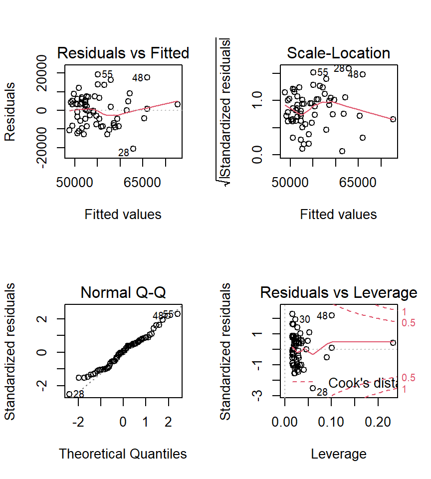
3.3.1 Diagnostic plots for simple regressions
Next, we want to obtain the base set of diagnostic plots that R makes available for ‘lm’ objects. This is the same set that we reviewed in the simple regression section of the course plus an additional normal probability plot of the residuals.
First for fit1:
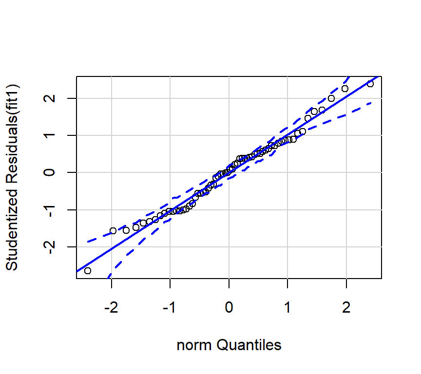
I prefer to draw the qqplot with the ‘qqPlot’ function from the ‘car’ package since it provides confidence bounds. See Fox and Weinberg (2011).
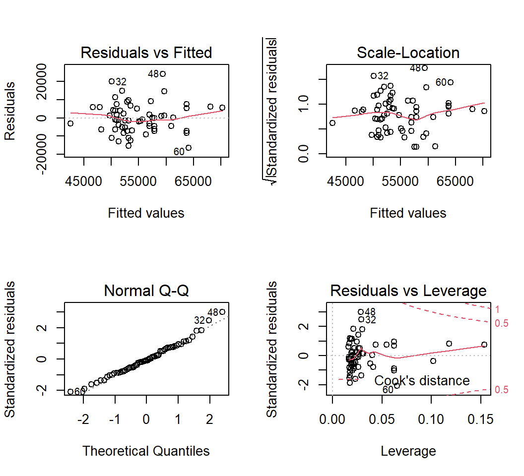
Next, the same plots for fit2:
And the preferred qqplot for fit2:
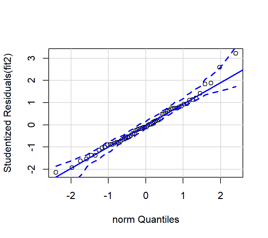
Since the tests of these two simple regression fits would not typically be used, the diagnostic plots would also not typically be of interest. The analyses seen above are largely here to put in place approaches and numeric values to compare the more interesting multiple regression results found below.