Chapter 4 Implementation of Standard Multiple Regression Analyses: Linear modeling with multiple IVs
When we covered implementation of simple regression procedures in R, we covered most of the R syntax required for multiple regression. Only a few additional coding strategies are necessary to employ models with more than one IV. We also reviewed those simple regression techniques in the previous section of this document. The illustrations outlined below emphasize a two-IV model for comparability to the example we worked out in SPSS. Some sections extend this capability to more than two IVs, but we will emphasize that to a greater degree at a later point in the course and in other documents.
The reader should also note that the following sections have two interrelated goals. One is simply the illustration of coding strategies in R for basic linear modeling. Some sections go beyond that narrow goal and continue to reinforce and expand the conceptual framework we have put in place for multiple regression. Some more advanced R strategies are also employed to obtain useful graphics and output that is formatted well for the markdown approach taken in this document.
The general sequence of the implementation is the following:
- perform the two-IV multiple regression
- obtain all the components and tests the we implemented in SPSS for the multiple regression
- obtain the basic evaluations of residual normality and homoscedasticity
- obtain additional information such as semi partial correlations, beta weights and CI’s
- reinforce the concepts of unique and common proportions of variance, R squared, SS partitioning, etc
- perform some diagnostics (topics not yet covered in lecture)
4.1 The core linear modeling approach with R
Requesting a multiple regression using lm is an easy extension of the basic expressions used for simple regression. The “model” specification still uses the “tilda” symbol to indicate the DV to the left and the IV’s to the right. All IV’s are named, and the plus symbol is used to essentially list the full set of IV’s. Here, I fit two models, each with the same two IVs, but I named them in opposite order. We will explore whether this makes any difference in outcome.
Typically we would NOT fit both models of the different IV orders. It is done here for instructional purposes that play out below and later in the semester.
First, establish the two alternative model fits:
4.1.1 Explore fit3 (salary~pubs+cits)
Obtain the same set of additional summaries/analyses/plots we did for simple regression. First for model fit3:
##
## Call:
## lm(formula = salary ~ pubs + cits, data = cohen1)
##
## Residuals:
##      Min       1Q   Median       3Q      Max
## -17133.1  -5218.3   -341.3   5324.1  17670.3
##
## Coefficients:
##             Estimate Std. Error t value Pr(>|t|)
## (Intercept) 40492.97    2505.39  16.162  < 2e-16 ***
## pubs          251.75      72.92   3.452  0.00103 **
## cits          242.30      59.47   4.074  0.00014 ***
## ---
## Signif. codes:  0 '***' 0.001 '**' 0.01 '*' 0.05 '.' 0.1 ' ' 1
##
## Residual standard error: 7519 on 59 degrees of freedom
## Multiple R-squared:  0.4195,	Adjusted R-squared:  0.3998
## F-statistic: 21.32 on 2 and 59 DF, p-value: 1.076e-07## 2.5 % 97.5 %
## (Intercept) 35479.6889 45506.2540
## pubs 105.8395 397.6605
## cits 123.3023 361.2931At this point, let’s recall the interpretation of the values for the regression coefficients. For comparison’s sake, analyses in the previous section found that when, in simple regression, salary was regressed on pubs, the regression coefficient was $350.80. It was interpreted to mean that each publication was related to an increase in salary of $350.80. Now, in the two-IV regression, the regression coefficient is seen to be $251.75. The change is recognized to have come about because the two IV’s are correlated and the multiple regression coefficient is said to be a partial regression coefficient. That is, it is the change in the DV for a one unit change in the IV, controlling for the presence of the other IV. So, in fit3, each pub is uniquely associated with about a $251.75 increase in salary. The interpretation of the regression coefficient for cits is similar. The conclusion is that the impact of each IV in a regression model is only interpretable in the context of that model. The presence or absence of other IV’s will influence the capability of any IV to predict the DV, when the IVs are correlate.
Next, we produce ANOVA summary tables two ways, using both the anova and Anova functions. Are they different?
Note that I have formatted the ANOVA tables in a manner that might be unfamiliar, using the ‘kable’ and ‘tidy’ functions. This approach permits direct comparison of the output from the two functions since the default listing for the ‘Anova’ table uses scientific notation for SS values. See the section below on R Markdown formatting capabilities for more detail on this.
The first thing to notice about the ANOVA tables found below is that they do not simply present SS Regression, SS Residual and SS total as you might have expected from how we saw that SPSS produced ANOVA tables. SS total is not shown at all, and SS Regression appears to be broken apart and assigned to the two IVs. Exactly where these SS for pubs and cits come from is a longer discussion. We covered this point earlier in our multiple regression expositions. Reiteration of the importance of this question is begun just below here and in an later section of this document (where we conceptually connect these SS to squared semi-partial correlations).
Make sure you see that the “statistic” column in the kable/tidy version of the ANOVA tables is actually just the F value. Make sure you know how these F’s were computed (what divided by what?)
| term | df | sumsq | meansq | statistic | p.value |
|---|---|---|---|---|---|
| pubs | 1 | 1472195326 | 1472195326 | 26.03841 | 0.0000037 |
| cits | 1 | 938602110 | 938602110 | 16.60086 | 0.0001396 |
| Residuals | 59 | 3335822387 | 56539362 | NA | NA |
# "unique" ss for each IV produced by this Anova function.
# Can also be found by multiplying
# the squared semi-partial for each IV by SStotal
kable(tidy(Anova(fit3,type="III")))# note this is Anova, not anova| term | sumsq | df | statistic | p.value |
|---|---|---|---|---|
| (Intercept) | 14769235188 | 1 | 261.22041 | 0.0000000 |
| pubs | 673921018 | 1 | 11.91950 | 0.0010337 |
| cits | 938602110 | 1 | 16.60086 | 0.0001396 |
| Residuals | 3335822387 | 59 | NA | NA |
At this point, in comparing the results from the two anova functions, it is useful to recall that anova produces Type I SS and Anova was set up to request Type III SS. For the moment, lets just note that the SS and F value for cits is the same in both anova tables. Cits was entered second in the model specification for fit3. This point is expanded below.
Next, we obtain the standard set of diagnostic plots are obtained as they were for simple regression. Recall that I ask for these plots to be put on one figure by using the ‘layout’ function. At this point in the course, we have not actually covered two of the four plots, but two are our standard assessments of the normality and homoscedasticity assumptions. There do not appear to be strong violations of either assumption (seen in the two plots on the left)
#influence(fit3)
# regression diagnostics
layout(matrix(c(1,2,3,4),2,2)) # optional 4 graphs/page
plot(fit3)
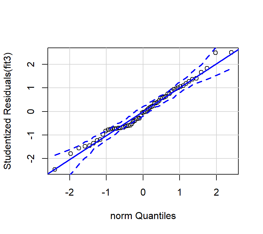
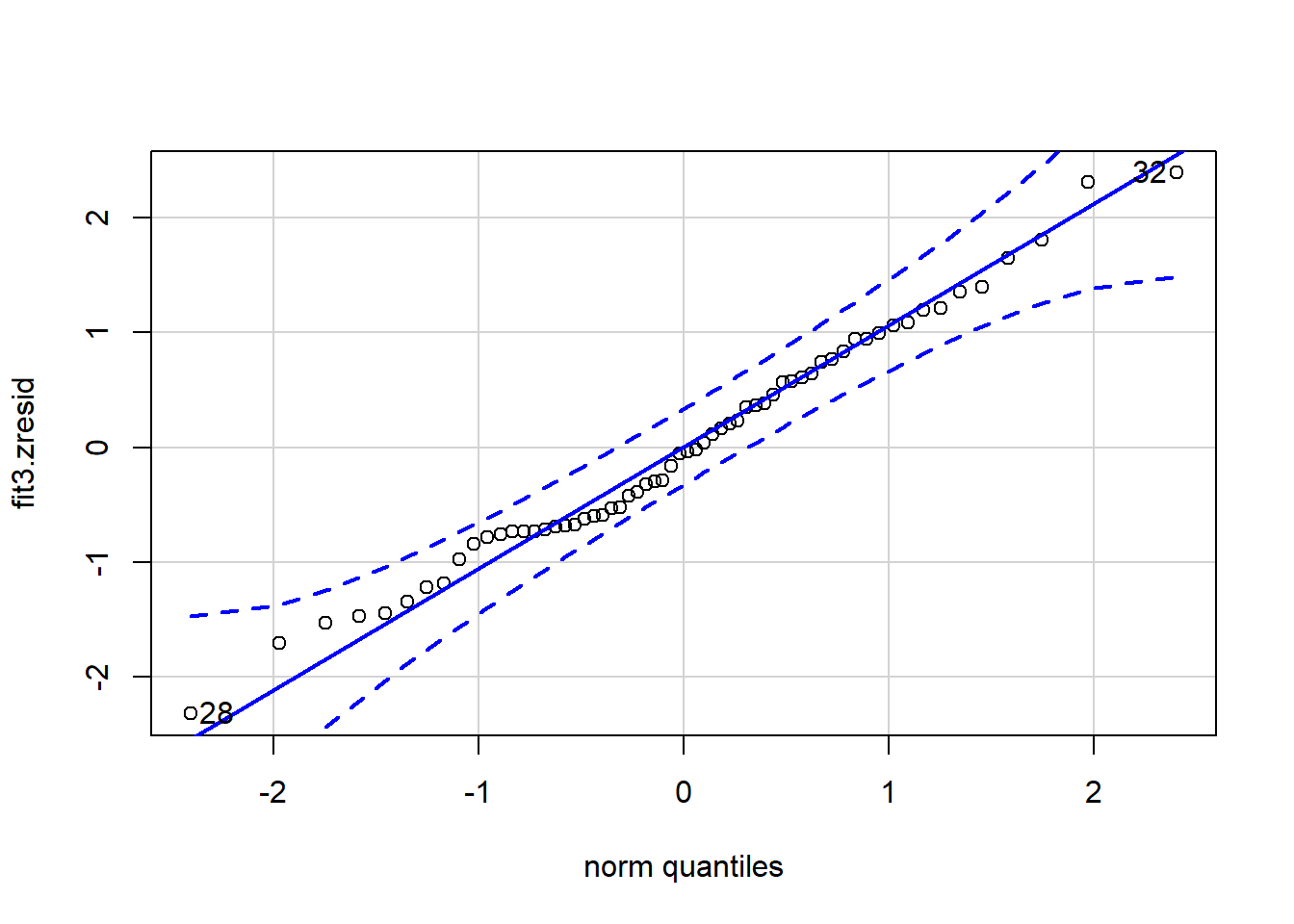
And we can also obtain the preferred qqplot:
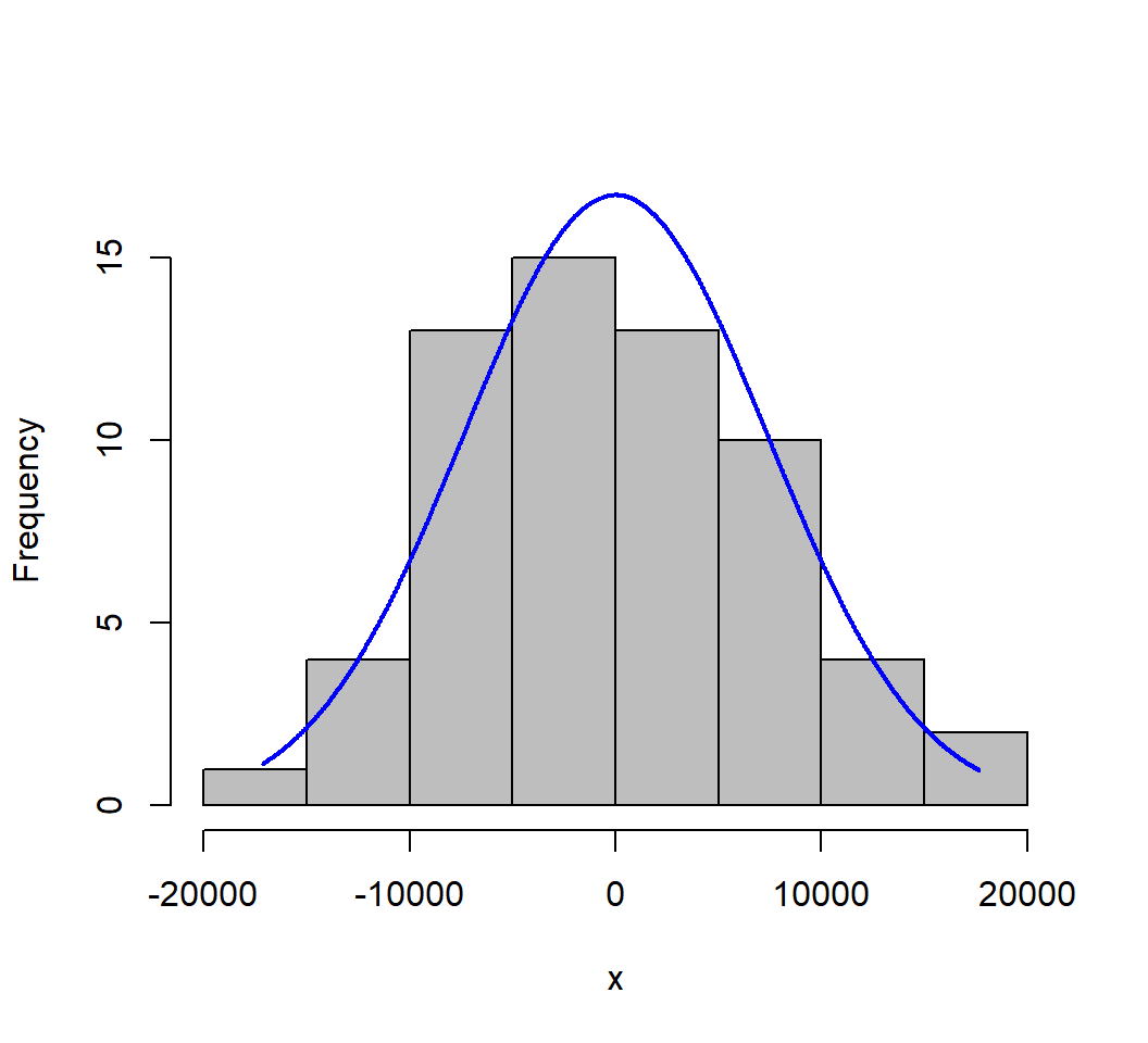
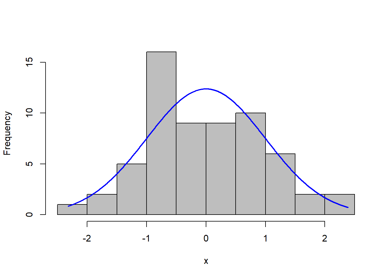
A histogram of the residuals with a normal curve overlaid also provides a helpful visualization.
4.1.2 Explore fit4 (salary~cits+pubs)
Next, we examine model fit4 (the one with the opposite order of IVs listed in the model specification):
##
## Call:
## lm(formula = salary ~ cits + pubs, data = cohen1)
##
## Residuals:
##      Min       1Q   Median       3Q      Max
## -17133.1  -5218.3   -341.3   5324.1  17670.3
##
## Coefficients:
##             Estimate Std. Error t value Pr(>|t|)
## (Intercept) 40492.97    2505.39  16.162  < 2e-16 ***
## cits          242.30      59.47   4.074  0.00014 ***
## pubs          251.75      72.92   3.452  0.00103 **
## ---
## Signif. codes:  0 '***' 0.001 '**' 0.01 '*' 0.05 '.' 0.1 ' ' 1
##
## Residual standard error: 7519 on 59 degrees of freedom
## Multiple R-squared:  0.4195,	Adjusted R-squared:  0.3998
## F-statistic: 21.32 on 2 and 59 DF, p-value: 1.076e-07## 2.5 % 97.5 %
## (Intercept) 35479.6889 45506.2540
## cits 123.3023 361.2931
## pubs 105.8395 397.6605The ANOVAS for fit4:
| term | df | sumsq | meansq | statistic | p.value |
|---|---|---|---|---|---|
| cits | 1 | 1736876419 | 1736876419 | 30.71977 | 0.0000007 |
| pubs | 1 | 673921018 | 673921018 | 11.91950 | 0.0010337 |
| Residuals | 59 | 3335822387 | 56539362 | NA | NA |
# "unique" ss for each IV produced by this Anova function.
# Can also be found by multiplying
# the squared semi-partial for each IV by SStotal
kable(tidy(Anova(fit4,type="III")))# note this is Anova, not anova| term | sumsq | df | statistic | p.value |
|---|---|---|---|---|
| (Intercept) | 14769235188 | 1 | 261.22041 | 0.0000000 |
| cits | 938602110 | 1 | 16.60086 | 0.0001396 |
| pubs | 673921018 | 1 | 11.91950 | 0.0010337 |
| Residuals | 3335822387 | 59 | NA | NA |
Once again, the SS and F’s are identical for pubs, which is the second IV specified in the model specification - is is the “last entered”. The SS and F’s differ for the first entered variable, cits, as was also the case for fit3. These differences are explored below.
We can also examine diagnostic plots for fit4. They should look identical to those for fit3 since the residuals are the same for each of the two fits.
#influence(fit3)
# regression diagnostics
layout(matrix(c(1,2,3,4),2,2)) # optional 4 graphs/page
plot(fit4)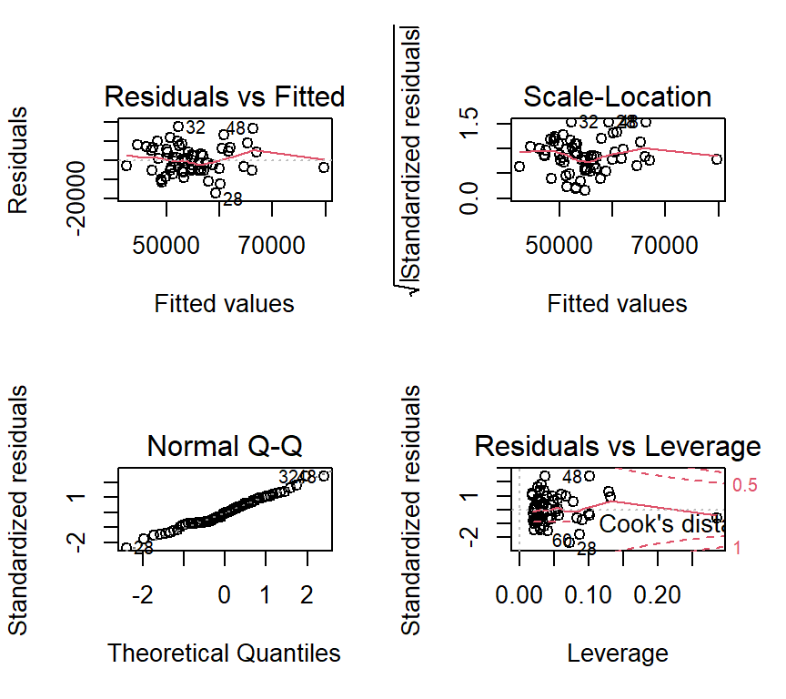
Here is the preferred qqplot for fit4:

4.1.3 Comparing fit3 and fit4 results.
We have emphasized how the SS and F-tests for fits 3 and 4 differ, depending on whether we use anova or Anova. But it is helpful to ask which components are identical for the two Fits. These items/statistics are identical:
- The Multiple R-squared
- SS Regression (although not printed above). It is found by adding the SS for the two IVs from the
anova-produced table. - SS Residual
- df regression/residual
- The regression coefficients, confidence Intervals, and t-tests of the coefficients are also identical for the two models
- Below, we also see that beta weights, partial r’s, semi-partial r’s, tolerances and unique/common variance proportions are identical for the two models
The primary difference emerges when examining the SS partitioning. Lets do one more comparison here. These SS computations will be revisited in a later chapter. If we rerun the fit3 model here it will permit comparing the SS, F’s and t-tests of the regression coefficients when using either anova or Anova. From this analysis, make note of the t-values. I saved them out of the model fit to work with in a section below.
##
## Call:
## lm(formula = salary ~ pubs + cits, data = cohen1)
##
## Residuals:
##      Min       1Q   Median       3Q      Max
## -17133.1  -5218.3   -341.3   5324.1  17670.3
##
## Coefficients:
##             Estimate Std. Error t value Pr(>|t|)
## (Intercept) 40492.97    2505.39  16.162  < 2e-16 ***
## pubs          251.75      72.92   3.452  0.00103 **
## cits          242.30      59.47   4.074  0.00014 ***
## ---
## Signif. codes:  0 '***' 0.001 '**' 0.01 '*' 0.05 '.' 0.1 ' ' 1
##
## Residual standard error: 7519 on 59 degrees of freedom
## Multiple R-squared:  0.4195,	Adjusted R-squared:  0.3998
## F-statistic: 21.32 on 2 and 59 DF, p-value: 1.076e-07## pubs cits
## 3.452463 4.074415Next, re-obtain the SS and F tests from the Anova function, and save the F values out to a vector.
## Anova Table (Type III tests)
##
## Response: salary
##                 Sum Sq Df F value    Pr(>F)
## (Intercept) 1.4769e+10  1 261.220 < 2.2e-16 ***
## pubs        6.7392e+08  1  11.919 0.0010337 **
## cits        9.3860e+08  1  16.601 0.0001396 ***
## Residuals   3.3358e+09 59
## ---
## Signif. codes: 0 '***' 0.001 '**' 0.01 '*' 0.05 '.' 0.1 ' ' 1## [1] 11.91950 16.60086Now we can take the square roots of the F values and compare those to the t values. Since each F is based on 1 and n-k-1 df, the square roots will produce a t value with those n-k-1 df.
## [1] 3.452463 4.074415## pubs cits
## 3.452463 4.074415Since the quantities are identical, we can conclude that the t-tests of the regression coefficients are equivalent to tests of Type III SS for each IV. Recalling comparisons of fit3 and fit4 above (the two opposite IV entry orders), we also recall that the coefficients and their t-tests are the same. The conclusion is that tests of the regression coefficients for any model are actually tests of type III SS for those IVs.
The type I SS seen from the anova analyses lead us to conclude that those SS are found by computing the unique SS for each variable at the point it enters the equation. That is why the SS for each variable differs, depending on whether it is entered first or second. The type III SS are found be treating each variable as if it were the second (last) to enter. Further implications of this are found in a later chapter.
4.1.4 Efficiently obtaining important descriptive components of a multiple-IV linear model
It has been argued that several core components of multiple regression should be produced whenever any linear model is fit. Some of those components have not yet been requested/produced with the methods outlined above (e.g. beta weights). I have written my own R function that obtains many of these additional items that we have previously discussed. The function is called mrinfo (multiple regression information) and I just call it Mr. Info. It is available in the bcdstats package.
The syntax is to just pass a lm model fit object to the mrinfo function. We do so here with our fit3 model and we will examine the output. The unique proportion of variance accounted for by each IV are equivalent to the square of the semi-partial correlation of that IV with the DV, after residualizing that IV on all other IVs. The argument minimal permits request of only a set of supplemental information or a longer list of regression information that has been covered above in piecemeal fashion.
## [[1]]
## NULL
##
## $`supplemental information`
##      beta wt structure r partial r semipartial r tolerances  unique  common
## pubs 0.36323     0.78145   0.40996       0.34245    0.88885 0.11727 0.13891
## cits 0.42867     0.84880   0.46860       0.40414    0.88885 0.16333 0.13891
##        total
## pubs 0.25618
## cits 0.30224
##
## $`var infl factors from HH:vif`
##    pubs    cits
## 1.12505 1.12505
##
## [[4]]
## NULL
We can obtain these statistics for fit4 as well, but all are identical to those from fit3.
## [[1]]
## NULL
##
## $`supplemental information`
##      beta wt structure r partial r semipartial r tolerances  unique  common
## cits 0.42867     0.84880   0.46860       0.40414    0.88885 0.16333 0.13891
## pubs 0.36323     0.78145   0.40996       0.34245    0.88885 0.11727 0.13891
##        total
## cits 0.30224
## pubs 0.25618
##
## $`var infl factors from HH:vif`
##    cits    pubs
## 1.12505 1.12505
##
## [[4]]
## NULL
The beta weights, partial correlations, semi-partial correlations, and tolerances should be values that the reader understands and expects, given our prior conceptual and SPSS work. But what are the “unique”, “common”, and “total” values. The reader should examine those, keeping in mind core ways of thinking about the Multiple R squared (which you know from above and from SPSS work). Recall that the multiple R-squared from both fits 3 and 4 was about .42. How might we describe the “unique” quantities, and how do they relate to the semi-partials? (Hint: sum the two unique proportions and add the common proportion)
4.1.4.1 A caveat on using ‘mrinfo’
The original data file from the cohen text called the “years since degree” variable “time”. We will examine a 3 IV model using that variable later in this document. At present, the word time can’t be used for a variable in a lm model that is submitted to the ‘mrinfo’ function. It thinks it is an R function called ‘time’. So I changed it to degree_yrs.
4.2 Diagnostic and Added-variable plots for the full two-IV model
Many graphical techniques can be explored for evaluation of assumptions, influence, and partial relationships in multivariable systems. A few are explored here, and others are presented in later chapters (e.g., see the chapter on the olsrr package).
4.2.1 Working with the residuals and predicted scores (yhats)
Residuals and yhats from any lm model can be quickly obtained.
These vectors can also be standardized.
We might also place these new vectors into a data frame along with the original variables, in order to save them for other future work.
# cohen1 was already detached
#detach(cohen1)
cohen1new <- cbind(cohen1, fit3.resid, fit3.pred, fit3.zresid, fit3.zpred)
# and then reattach cohen1 for possible use later
#attach(cohen1new)
Now we can work directly with these new residual and yhat vectors. Some of these plots duplicate what was shown above, but it is useful to have the standardized residuals and yhats available.
## [1] 32 28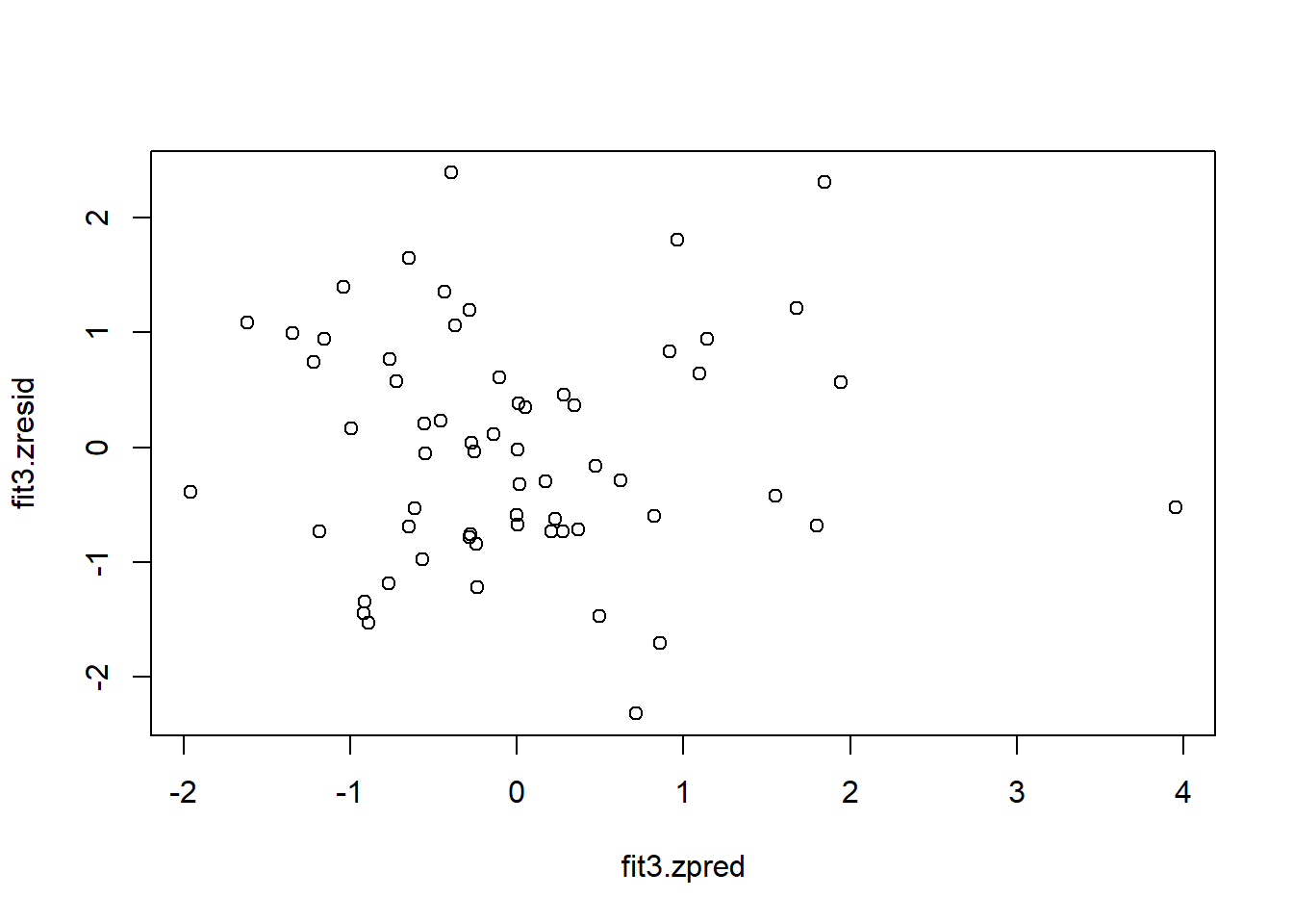
Now detach the cohen1new data frame and reattach the original to be used later.
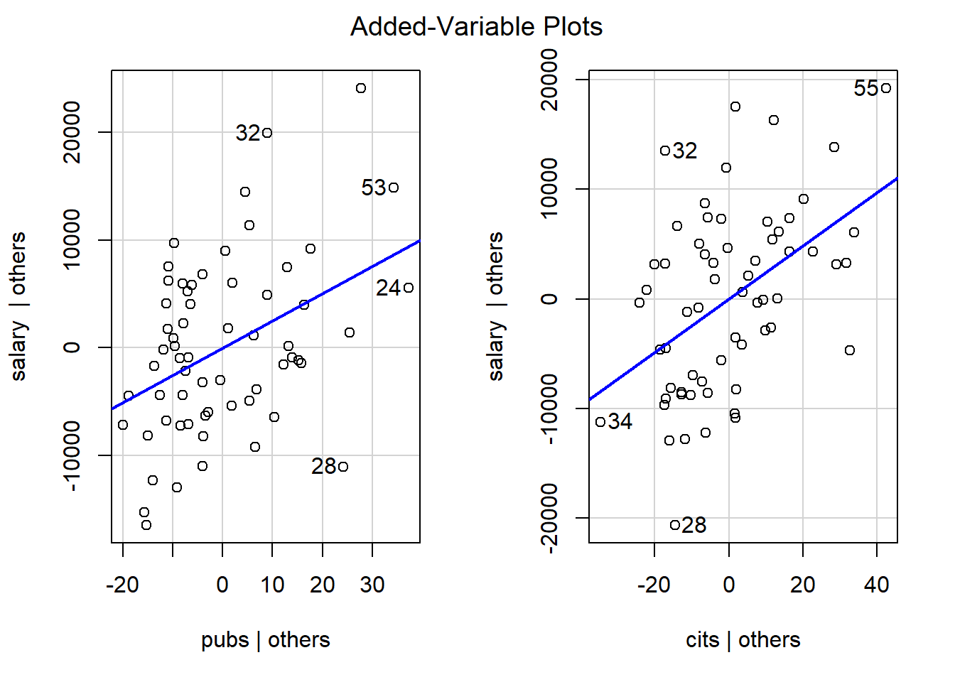
4.2.2 Added Variable Plots
Added variable plots permit evaluation of the so-called partial regressions. These are actually just plots of the partial correlations of each IV (residualized on the other IVs) with Y (also residualized on the other IV). Note that the “test” of these partial correlations is equivalent to the test of the semi-partial correlations and also equivalent to the tests of the individual regression coefficients found in the summary output.
See the later chapters on Extensions and use of the olsrr package for further treatment of this.