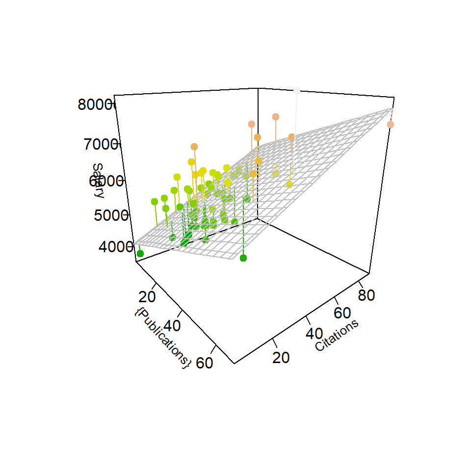
Chapter 8 Examine the fit of the plane in a 3D wireframe plot:
R has useful facilities for creating a three dimensional scatter plot. It is also possible to plot the model fit onto that 3D scatter plot. The two-IV model fits a plane. This section creates the model, generates the scatter plot, adds the plane, and permits rotation of the plot if the code is executed in R or RStudio.
Initially we have to relabel the variables in order to use the 3d scatter plot function below.
# to simplify the use of the scatter3D function, we re-label the variables.
# scatter3D expects the "Y" variable from a linear model to be in the "z" dimension of the 3D plot
z <- cohen1$salary
x <- cohen1$pubs
y <- cohen1$cits
# Again fit the two-IV model, but using the x,y,z variables
# x,y, and z are used for purposes related to the 3D surfce plotting below.
# This model is the same as fit3 examined above
fit3d1 <- lm(z~x+y)
#summary(fit.dep1b)
tidyfit.3d1 <- tidy(fit3d1) # nicer table than with summary
kable(tidyfit.3d1, format="markdown")| term | estimate | std.error | statistic | p.value |
|---|---|---|---|---|
| (Intercept) | 40492.9715 | 2505.39437 | 16.162314 | 0.0000000 |
| x | 251.7500 | 72.91896 | 3.452463 | 0.0010337 |
| y | 242.2977 | 59.46809 | 4.074415 | 0.0001396 |
Drawing the 3d scatter plot is somewhat complicated and the student in 510/511 is not expected to master the code at this point. However, one should be able to take this code and modify it to be used in and two-IV model fit with other data sets.
In order to draw the 3D scatter plot we need to do the following:
- Set up a grid of hypothetical points along a plane (I chose 21 lines for visual style reasons). The grid is established with minimal and maximal values in the x and y dimensions by using the minimal and maximal values for the x and y variables (pubs and cits in our case)
- Create a matrix of predicted scores (in the y scale), using the prediction equation that we called fit3d1 above.
- use the ‘scatter3D’ function from the ‘plot3D’ package. This draws the basic scatter plot, permits some color control of points, allows text and label editing, and permits addition of a surface.
# set up a grid required for the plane drawn by the surface argument of scatter3D
grid.lines = 21
x.pred <- seq(min(x), max(x), length.out = grid.lines)
y.pred <- seq(min(y), max(y), length.out = grid.lines)
xy <- expand.grid( x = x.pred, y = y.pred)

z.pred <- matrix(predict(fit3d1, newdata = xy),
                 nrow = grid.lines, ncol = grid.lines)
# fitted points for droplines to surface if we want to draw them
fitpoints <- predict(fit3d1)
This 3D scatter plot capability is useful in one important manner not demonstrated in the html or pdf versions of this document. If the code is run in R (preferable RStudio), the ‘scatter3D’ function can be followed by a ‘plotrgl’ function (commented out here). This will pop up a graphics window and the user can use the mouse to manually rotate the 3D image. This provides superb visualization capability. In the scatter3D implementation here the theta and phi values are chosen to produce what I thought was the best rendition of the 3D image for the 2 dimensional rendering required for print documents.
# scatter plot with regression plane
scatter3D(x, y, z, pch = 20, cex = 1.5, cex.lab=.8,
          theta = 50, phi = 20, ticktype = "detailed",
#          theta = 50, phi = 18, ticktype = "detailed",
          zlim=c(35000, 82000),
          #cex.axis=.9,
          xlab = "{Publications}", ylab = "Citations",
          zlab = "Salary",
          surf = list(x = x.pred, y = y.pred, z = z.pred,
                      facets = NA,
                      col="grey75",
                      fit = fitpoints),
          colkey=F, col=terrain.colors(length(z)),
          main = "",
          plot=T)