Chapter 12 Resampling and Robust methods for Linear Models
Two classes of alternative approaches to linear modeling are breifly described in this section. The first is bootstrapping which is an alternative to std error calculation when faced with non-normal residuals. Although there are many “flavors” of bootstrapping, only two are illustrated here. The second class is a broad range of methods falling under the rubric of Robust Regression. The ones emphasized here are those that can help when heteroscedasticity is present in an OLS model. The code is not accompanied by much commentary or explanation. It is presumed that background on bootstrapping methods is obtained elsewhere.
12.1 Ordinary nonparametric bootstrapping with the boot function
The boot package has extensive facilities for bootstrapping many kinds of analyses. The essential logic is to tell the boot function which statistic from the analysis needs to be bootstrapped, what kind of bootstrapping (e.g., casewise vs residual), and then requests for summaries of the bootstrapping. This first section is based somewhat on the methods outlined in the Quick-R website [https://www.statmethods.net/advstats/bootstrapping.html]. The methods presented here are nonparametric bootstrapping methods.
Each statistic of interest can be bootstrapped. But this requires writing a function to extract that statistic from the lm fit so that it can be repeated with the bootstrap samples. This section will do bootstrap analyses on three statistics:
- The Multiple R-Squared from the two-IV model used throughout this doc.
- The pvalue for the F test of that Multiple R-squared (test of the “whole” equation).
- The regression coefficients from the two-IV equation.
In these illustrations, I ran the boot function (creating the results object) within a call to the system.time function to record how long it took to do the bootstrap resampling. This will vary across platforms.
12.1.1 Bootstrap the multiple R-squared statistic
#library(boot)
# Bootstrap 95% CI for R-Squared
# function to obtain R-Squared from the data
multrsq <- function(formula, data, indices) {
     d <- data[indices,] # allows boot to select sample
     fit <- lm(formula, data=d)
     return(summary(fit)$r.square)
}
# bootstrapping with 2000 replications
# for other kinds of statistics, `boot` may need a "maxit" argument to  set the upper limit on iterations
set.seed(1234) # for reproducibility within this document
system.time(results1 <- boot(data=cohen1, statistic=multrsq,
   R=2000, formula=salary~pubs+cits))
## user system elapsed
## 1.64 0.00 1.64##
## ORDINARY NONPARAMETRIC BOOTSTRAP
##
##
## Call:
## boot(data = cohen1, statistic = multrsq, R = 2000, formula = salary ~
## pubs + cits)
##
##
## Bootstrap Statistics :
## original bias std. error
## t1* 0.4195157 0.0118493 0.09665115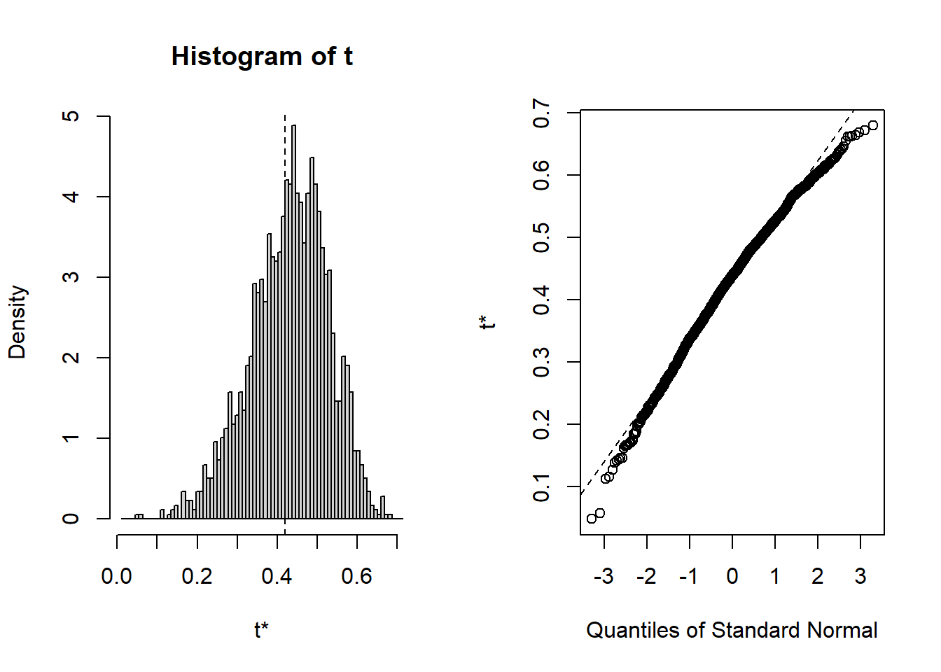
## BOOTSTRAP CONFIDENCE INTERVAL CALCULATIONS
## Based on 2000 bootstrap replicates
##
## CALL :
## boot.ci(boot.out = results1, type = c("norm", "basic", "perc",
##     "bca"))
##
## Intervals :
## Level      Normal              Basic
## 95%   ( 0.2182,  0.5971 )   ( 0.2378,  0.6161 )
##
## Level     Percentile            BCa
## 95%   ( 0.2230,  0.6013 )   ( 0.1806,  0.5768 )
## Calculations and Intervals on Original Scale
12.1.2 Bootstrap the omnibus F test p value
fpval <- function(formula, data, indices) {
     d <- data[indices,] # allows boot to select sample
     fit <- lm(formula, data=d)
     return(pf(summary(fit)$fstatistic[1],
               df1=summary(fit)$fstatistic[2],
               df2=summary(fit)$fstatistic[3],lower.tail=F))
}
# bootstrapping with 2000 replications
# for other kinds of statistics, `boot` may need a "maxit" argument to  set the upper limit on iterations
set.seed(1234) # for reproducibility within this document
system.time(results2 <- boot(data=cohen1, statistic=fpval,
   R=2000, formula=salary~pubs+cits))
## user system elapsed
## 2.03 0.00 2.03##
## ORDINARY NONPARAMETRIC BOOTSTRAP
##
##
## Call:
## boot(data = cohen1, statistic = fpval, R = 2000, formula = salary ~
## pubs + cits)
##
##
## Bootstrap Statistics :
## original bias std. error
## t1* 1.076015e-07 0.0003175022 0.006625147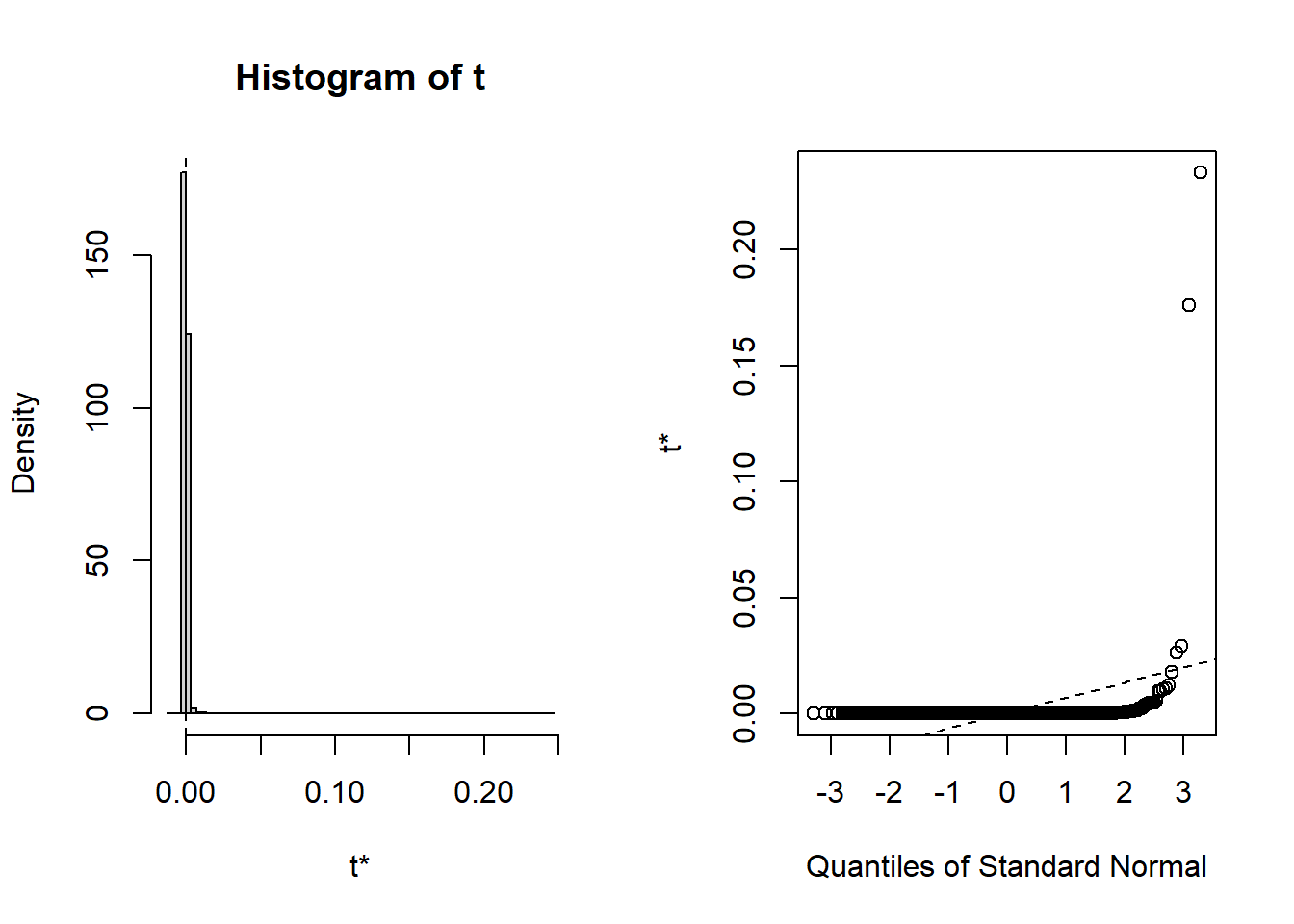
## BOOTSTRAP CONFIDENCE INTERVAL CALCULATIONS
## Based on 2000 bootstrap replicates
##
## CALL :
## boot.ci(boot.out = results2, type = c("bca"))
##
## Intervals :
## Level       BCa
## 95%   ( 0.0000,  0.0041 )
## Calculations and Intervals on Original Scale
12.1.3 Bootstrap the regression coefficients
Next, we will bootstrap the regression coefficients
# Bootstrap 95% CI for regression coefficients
#library(boot)
# function to obtain regression weights
coeffs <- function(formula, data, indices) {
  d <- data[indices,] # allows boot to select sample
  fit <- lm(formula, data=d)
  return(coef(fit))
}
# bootstrapping with 2000 replications
# for other kinds of statistics, `boot` may need a "maxit" argument to  set the upper limit on iterations
set.seed(1234) # for reproducibility within this document
system.time(results3 <- boot(data=cohen1, statistic=coeffs,
        R=2000, formula=salary~pubs+cits))
## user system elapsed
## 1.36 0.00 1.36##
## ORDINARY NONPARAMETRIC BOOTSTRAP
##
##
## Call:
## boot(data = cohen1, statistic = coeffs, R = 2000, formula = salary ~
## pubs + cits)
##
##
## Bootstrap Statistics :
## original bias std. error
## t1* 40492.9715 -92.356087 2481.39738
## t2* 251.7500 -2.286656 85.13455
## t3* 242.2977 2.522431 58.03025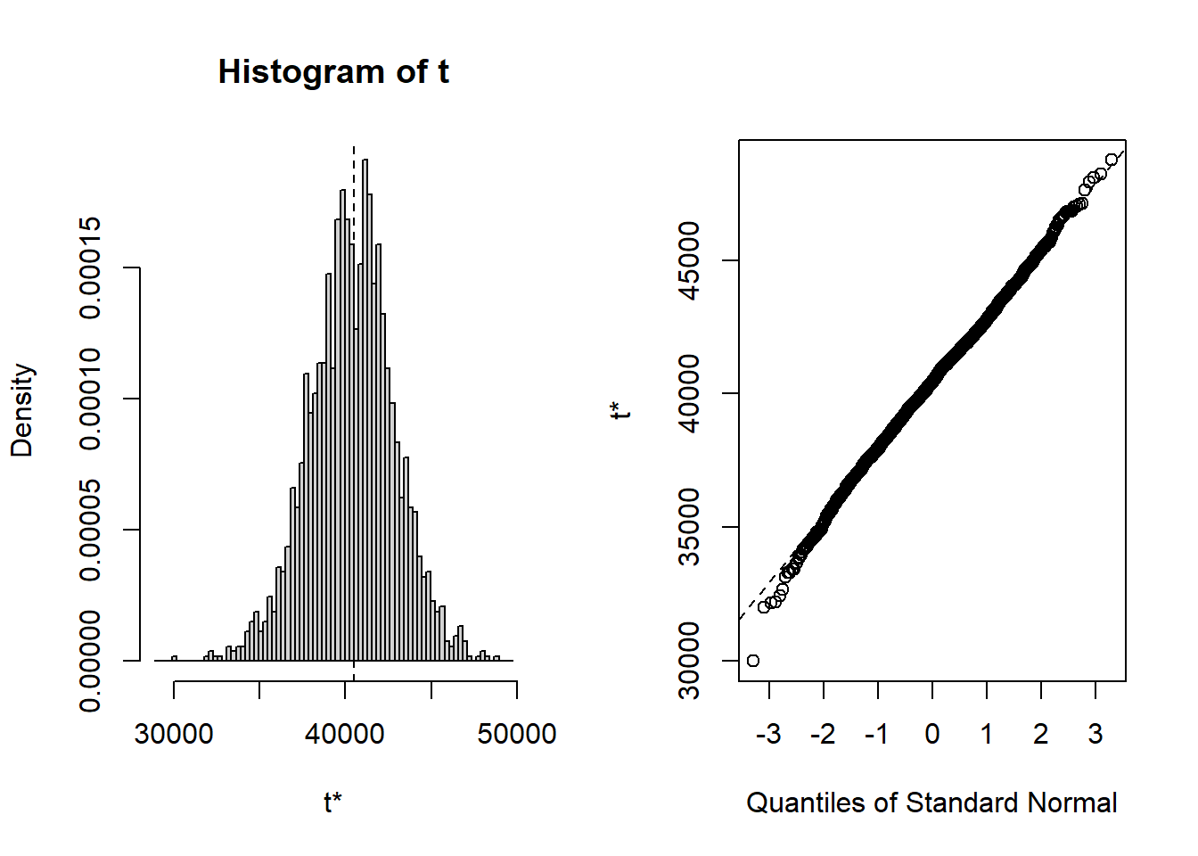


## BOOTSTRAP CONFIDENCE INTERVAL CALCULATIONS
## Based on 2000 bootstrap replicates
##
## CALL :
## boot.ci(boot.out = results3, type = "bca", index = 1)
##
## Intervals :
## Level       BCa
## 95%   (35539, 45437 )
## Calculations and Intervals on Original Scale## BOOTSTRAP CONFIDENCE INTERVAL CALCULATIONS
## Based on 2000 bootstrap replicates
##
## CALL :
## boot.ci(boot.out = results3, type = "bca", index = 2)
##
## Intervals :
## Level BCa
## 95% ( 86.9, 424.7 )
## Calculations and Intervals on Original Scale## BOOTSTRAP CONFIDENCE INTERVAL CALCULATIONS
## Based on 2000 bootstrap replicates
##
## CALL :
## boot.ci(boot.out = results3, type = "bca", index = 3)
##
## Intervals :
## Level BCa
## 95% (112.6, 340.1 )
## Calculations and Intervals on Original Scale12.2 An alternative bootstrap approach from car package functions
John Fox has produce the car package that we have seen contains many useful functions for linear modeling (Fox, 2016). One function, Boot, provides a flexible approach to non-parametric bootstrapping that may be easier to use. I also find that the Confint function is a quicker way to get a full picture of bootstrapped confidence intervals.
# Bootstrap 95% CI for regression coefficients
#library(boot)
# function to obtain regression weights
coeffs <- function(formula, data, indices) {
  d <- data[indices,] # allows boot to select sample
  fit <- lm(formula, data=d)
  return(coef(fit))
}
# bootstrapping with 2000 replications
# for other kinds of statistics, `boot` may need a "maxit" argument to  set the upper limit on iterations
set.seed(1234) # for reproducibility within this document
system.time(results4 <- Boot(fit3, f=coef,
        R=2000, method=c("case"))) # can specify casewise or residual sampling with the method argument
## user system elapsed
## 1.40 0.00 1.41##
## Number of bootstrap replications R = 2000
## original bootBias bootSE bootMed bootSkew bootKurtosis
## (Intercept) 40492.97 -92.3561 2481.397 40430.85 -0.1058512 0.314662
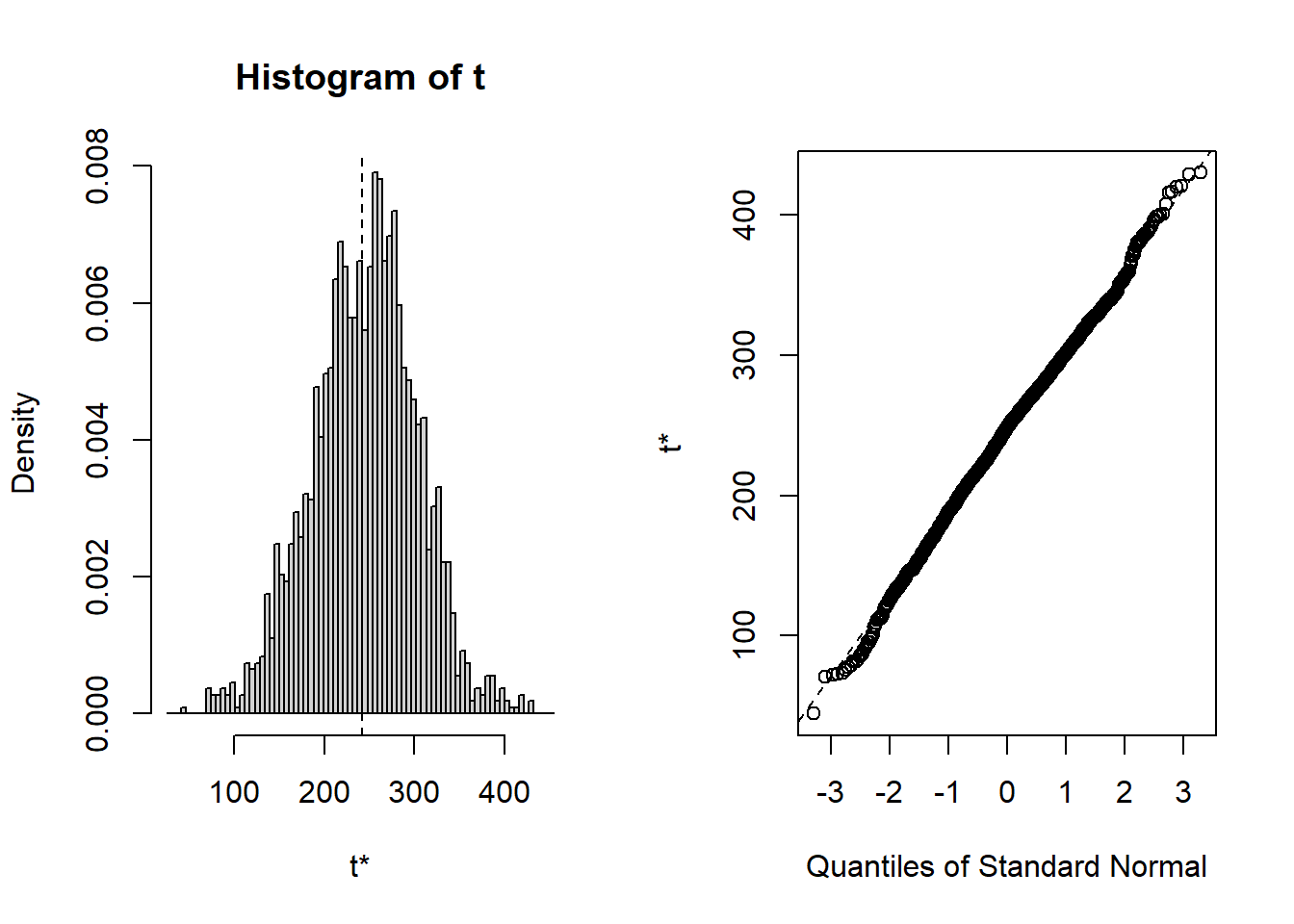
## pubs 251.75 -2.2867 85.135 248.05 0.0016417 0.013766
## cits 242.30 2.5224 58.030 248.02 -0.1261283 0.134424Bootsrapped empirical distributions for each coefficient are produced with the application of the base system plot function to the bootstrapped results.


And confidence intervals of multiple types are readily produced. Percentile (“perc”) and “bca” are typically recommended.
## Bootstrap normal confidence intervals
##
##               Estimate       2.5 %     97.5 %
## (Intercept) 40492.9715 35721.87804 45448.7770
## pubs          251.7500    87.17604   420.8973
## cits 242.2977 126.03808 353.5125## Bootstrap percent confidence intervals
##
## Estimate 2.5 % 97.5 %
## (Intercept) 40492.9715 35280.22022 45274.3103
## pubs 251.7500 77.56269 415.7893
## cits 242.2977 127.95169 353.4045## Bootstrap bca confidence intervals
##
## Estimate 2.5 % 97.5 %
## (Intercept) 40492.9715 35539.48858 45436.7048
## pubs 251.7500 86.91784 424.6978
## cits 242.2977 112.56818 340.1057# obtain a useful set of histograms for each coefficient distribution
hist(results4, legend="separate")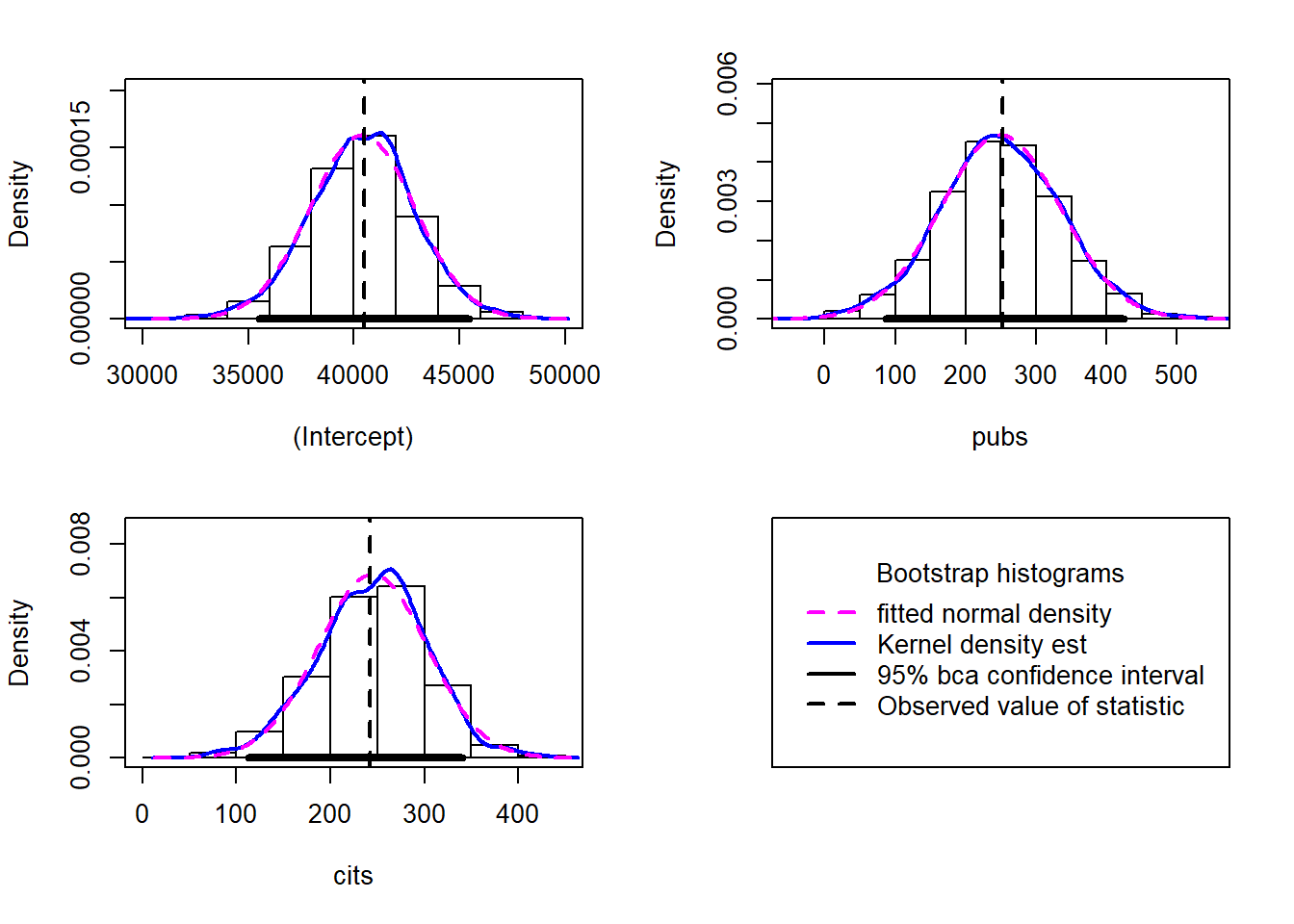
##             (Intercept)       pubs        cits
## (Intercept)  6157332.98 -47605.756 -112384.905
## pubs          -47605.76   7247.891   -1593.342
## cits         -112384.90  -1593.342    3367.510
12.3 Robust Regression for heteroscedastic data sets
Bootstrapping methods are primarily employed as a tool to handle situations where normality assumptions are violated. They are not necessarily insensitive to heteroscedasticity issues. In this section, I outline tools available from the car, lmtest, MASS, and sandwich packages for robust regression analyses. Also included is a brief introduction to a suite of robust methods for handling data sets with outliers and influential cases.
12.3.1 A robust Standard Errors approach from the car Package when heteroscedasticity is present.
The Salary-pubs-cits data set was not one that showed much heteroscedasticity, so submitting it to robust methods may not be necessary. Another data set we have see previously does have heteroscedasticity and this is what is used here. This is a data set provided by Dr. James Boswell on baseline scores of anxiety-diagnosed patients on scales of depression severity (bods, treated as the DV), anxiety severity (boasev), and positive affect (bpa). A standard two-IV linear model is fit and then corrected.
The two-iv regression produced a multiple R-squared of about .42 and the standard tests of the two IVs are shown here. Note that the data set has a fairly large N (200) and thus substantial power for effects of the size seen.
fit10<- lm(bods~boasev+bpa, data=boswell)
kable(tidy(fit10), caption=
"Regression Coefficients and Regular Parametric Std Errors")| term | estimate | std.error | statistic | p.value |
|---|---|---|---|---|
| (Intercept) | 5.7363514 | 1.6676431 | 3.439796 | 0.0007105 |
| boasev | 0.5829990 | 0.0775505 | 7.517665 | 0.0000000 |
| bpa | -0.2104816 | 0.0405446 | -5.191359 | 0.0000005 |
The plot of residuals vs yhats reveals an odd pattern, that reflects a truncated variable (boasev). But it also reveals a modest amount of heteroscedasticity.
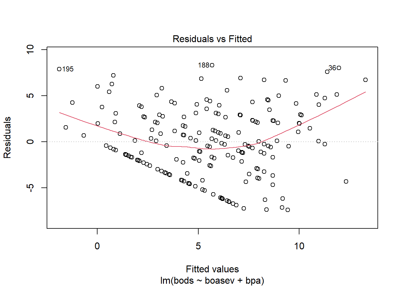
Testing a null hypothesis of no heteroscedasticity with the Breusch-Pagan test finds a p value in the rejection range.
##
## 	studentized Breusch-Pagan test
##
## data:  fit10
## BP = 16.966, df = 2, p-value = 0.0002069
Several different methods of estimating corrected covariance matrices based on heteroscedasticity are available. The one illustrated here (“HC0”) is often simply called the White Std Error. See the help doc on hccm for more details. The hccm function is from the car package and coeftest is from the lmtest package. You can see that the standard errors are different than the regular standard errors, but they are not much larger owing to the fact that heteroscedasticity is not severe in this data set.
cov <- hccm(fit10, type="hc0") #needs package 'car'
fit10.HC0 <- coeftest(fit10, vcov.=cov)
kable(tidy(fit10.HC0), caption=
"Robust (HC0) standard errors and modified t-tests")| term | estimate | std.error | statistic | p.value |
|---|---|---|---|---|
| (Intercept) | 5.7363514 | 1.9687184 | 2.913749 | 0.0039840 |
| boasev | 0.5829990 | 0.0984717 | 5.920470 | 0.0000000 |
| bpa | -0.2104816 | 0.0454911 | -4.626872 | 0.0000067 |
12.3.2 The Wald test and an alternative to adjusted t-tests for linear models with heteroscedasticity
The lmtest package has a function called waldtest that permits a commonly used inferential method, the Wald Test, which also employs covariance matrix correction for heteroscedasticity. It uses a model comparison strategy. First we created an intercept only model (mod0) and the the full two-IV model (modfull). waldtest then compares those two models in a standard model comparision methodology and the F test evalutes the improvement in fit, but using corrected standard errors of the White type (HC0). This F value is somewhat smaller than the one seen above for the regular OLS method, and is the alternate method for testing the null about the overall fit of the model. The vcovHC function comes from the sandwich package and is a common one for estimating the covariance structure in the presence of heteroscedasticity.
#library(lmtest)
#library(sandwich)
mod0 <- lm(bods~1 , data=boswell)
modfull <- lm(bods~boasev+bpa , data=boswell)
waldtest(mod0, modfull, vcov = vcovHC(modfull, type = "HC0"))
## Wald test
##
## Model 1: bods ~ 1
## Model 2: bods ~ boasev + bpa
## Res.Df Df F Pr(>F)
## 1 199
## 2 197 2 57.232 < 2.2e-16 ***
## ---
## Signif. codes: 0 '***' 0.001 '**' 0.01 '*' 0.05 '.' 0.1 ' ' 1The lmtest package also has a function to test the individual regression coefficients with the adjusted standard errors. This approach is identical to the one shown above with the car package tools. The vcovHC function comes from the lmtest package. Adjusted standard errors and t’s are the same as above since the same White Std. Errors are chosen.
#library("lmtest")
#library("sandwich")
# Robust t test
coeftest(modfull, vcov = vcovHC(modfull, type = "HC0"))
##
## t test of coefficients:
##
## Estimate Std. Error t value Pr(>|t|)
## (Intercept) 5.736351 1.968718 2.9137 0.003984 **
## boasev 0.582999 0.098472 5.9205 1.406e-08 ***
## bpa -0.210482 0.045491 -4.6269 6.719e-06 ***
## ---
## Signif. codes: 0 '***' 0.001 '**' 0.01 '*' 0.05 '.' 0.1 ' ' 112.4 Robust regression methods when outliers or highly influential cases are present
When outliers or highly influentical cases are detected via influence analysis it is possible to use that information to refine the linear model. The general idea is to take an influence statistic such as Cook’s D and use it to weight the importance of cases in the regression. One commonly recommended method is called “Iteratively Reweighted Least Squares”. The rlm function in the MASS package is a recommended method to perform such weighted/reweighted least squares. Rather than take additional space in this document, the reader is referred to a very good tutorial page on IRLS using rlm. This tutorial page is from the UCLA Statistical Consulting unit which has created many useful tutorials.