Chapter 11 Regression diagnostics and Influence Analysis
In a future section of the course, we will look more carefully at procedures for diagnosing problem issues in linear model fits, including the violation of assumptions. We will also build concepts that address how influential specific cases and variables are for the particular outcome that our linear modeling produces. This section of the current document will simply present code for a long list of these things without much comment, annotation, or explanation. It serves to put these capabilities in place for the point in time when we will need them The illustrations are all based on the fit3 model evaluated above:
11.1 A set of standard influence and diagnostic statistics
Several indices are calculated here that produce values for each case in the data set. I show how, with subsetting, to obtain individual case values for some of these (dfbetas and dffits), but don’t print all values for any of them. The last code line in this chunk reminds us how to use headtail to examine the first few and last few elements of an object - dfbetas are shown.
#  Diagnostics
#  create the whole suite; look at each by doing, e.g., print(sresids)
sresids <- rstandard(fit3) #store the standardized residuals in a variable named "sresids"
standresid <- stdres(fit3) #store the standardized residuals in a variable named "standresids"
stud.del.resids <- rstudent(fit3) #store the studentized deleted residuals in a variable named "stud.del.resids"
leverage_hats <- hatvalues(fit3) #get the leverage values (hi)
cooksD <- cooks.distance(fit3) #get Cook's distance
dfbetas <- dfbetas(fit3) #calculate all dfbetas
dfbetas_4_0 <- dfbetas(fit3)[4,1] #dfbeta for case 4, first coefficient (i.e., b_0)
dffits <- dffits(fit3) #All dffits
dffits_4 <- dffits(fit3) [4] #dffits for case 4
influence <- influence(fit3) #various influence statistics, including hat values and dfbeta (not dfbetas) values
# examine dfbetas, for example
headtail(dfbetas)
## (Intercept) pubs cits
## 1 0.0081286885 0.019596957 -0.055510624
## 2 0.1608435212 -0.105631169 -0.061098985
## 3 0.0009316857 -0.007992130 0.005670943
## ...
## 59 -0.0742222603 0.056792584 0.011273927
## 60 0.2251262055 0.277341258 -0.484391375
## 61 -0.1449618287 -0.126384177 0.158434883
## 62 0.2185338279 -0.150682252 -0.072804543Variance Inflation factors are useful indices for assessing multicolinearity. In a two-IV model such as this one, these will not be very interesting unless the two IVs are extremely highly correltated. And for a two-IV model the VIFs will be the same for each IV, since there is only one other IV to be correlated with for each of them (and it is the same correlation). So, this illustration is not very informative beyond showing how to obtain the VIFs.
#library(car) #load the package car if not still loaded from above
vif <- vif(fit3) #variance inflation factors
vif
## pubs cits
## 1.12505 1.12505## pubs cits
## 1.060684 1.060684## pubs cits
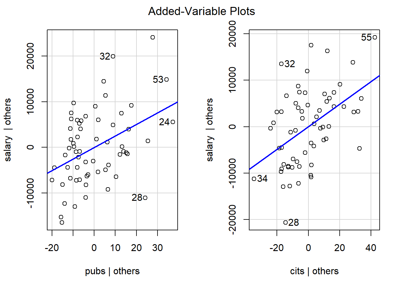
## FALSE FALSEAdded variable plots are a tool that permits examination of the partial correlations between pairs of variables. Each of the two variables in a plot has been residualized on all other variables.
This code chunk creates a plot of Cooks D values (an influence statistic) as a function of sequential case number in the data set. It also identifies extreme cases (case numbers labeled) based on a threshold set in the threshold object. As discussed in class, it is best to look for Cook’s D values divergent from others rather than those exceeding a numerical criterion, but some criteria have been proposed and one of those defines the threshold here.
# Cook's D plot
# identify D values > 4/(n-k-1)
threshold  <- 4/((nrow(cohen1)-length(fit3$coefficients)-2))
plot(fit3, which=4, cook.levels=threshold)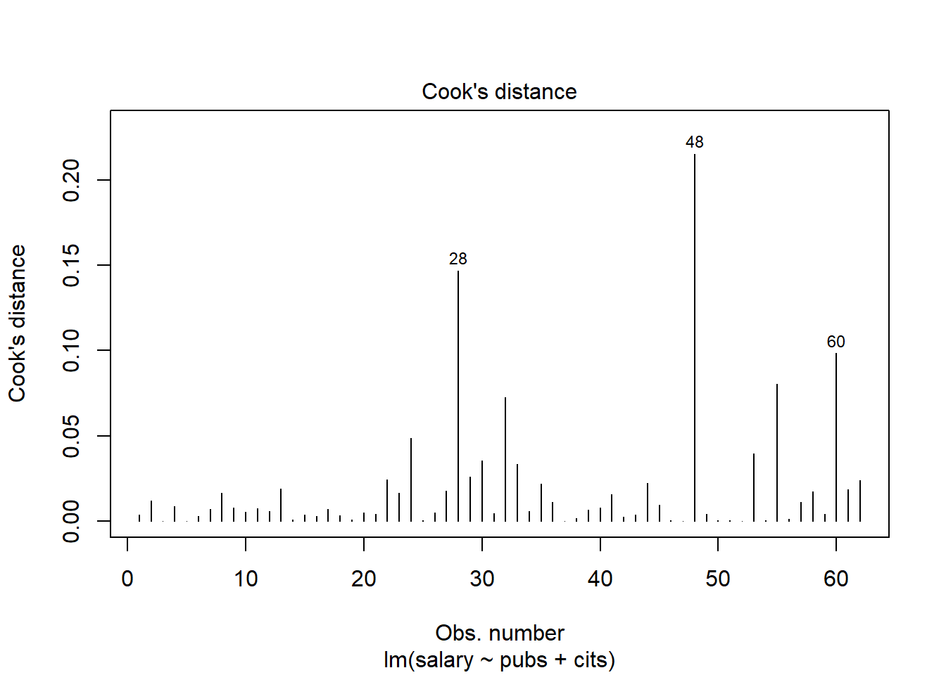
This influence plot is a standard scatterplot of residuals against yhats, and is the plot used to visually assess heteroscedasticity. But the added benefit here is that the size (area) of each point is scaled to the Cook’s D statistic thus permitting a visualization of the most influential cases in their residual/yhat position.
# Influence Plot
influencePlot(fit3, id=TRUE,
              main="Influence Plot", sub="Circle area is proportial to Cook's Distance" )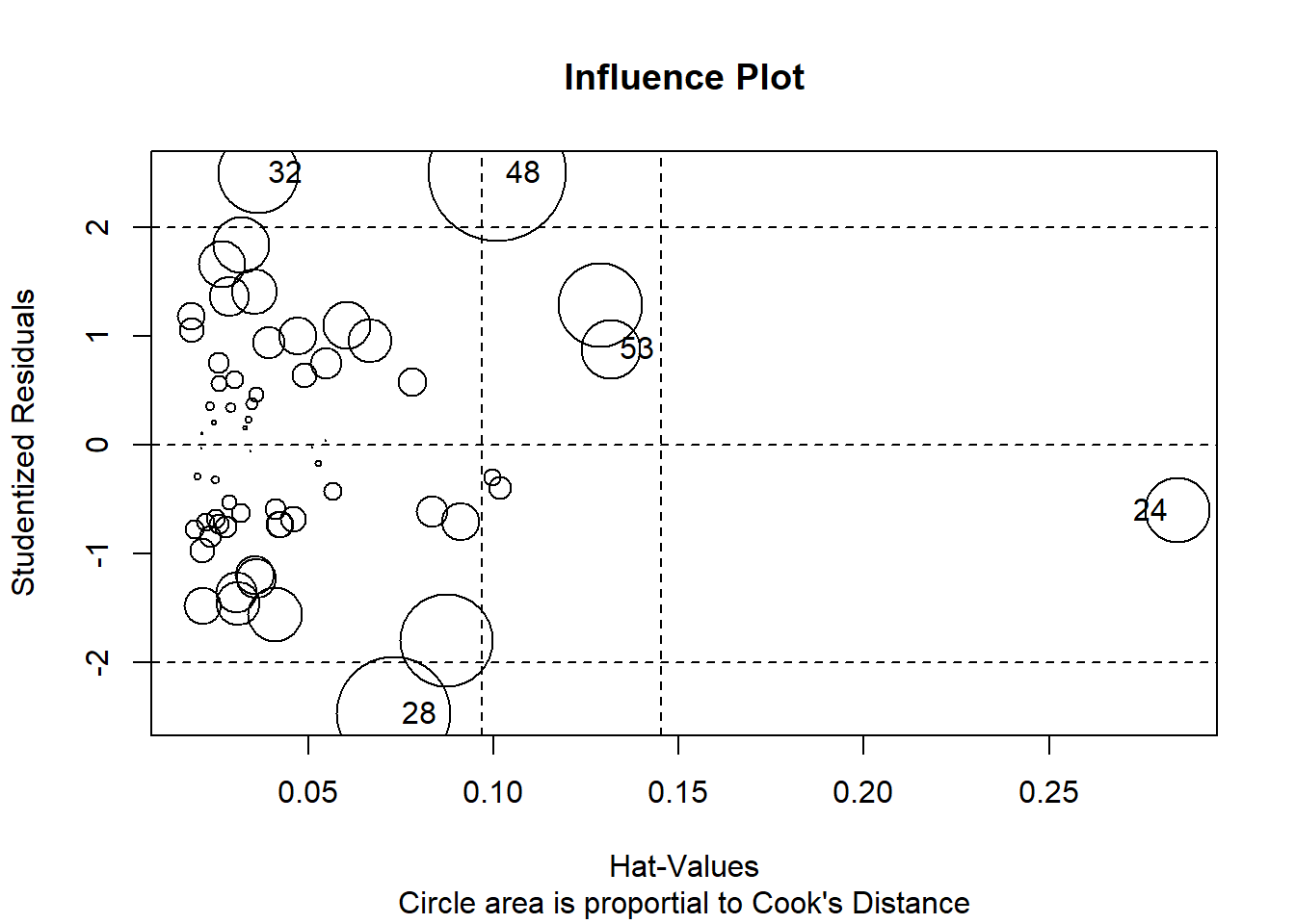
##       StudRes        Hat      CookD
## 24 -0.6018576 0.28463388 0.04856737
## 28 -2.4663093 0.07292105 0.14683221
## 32  2.4982801 0.03657164 0.07253089
## 48  2.5025997 0.10097428 0.21527380
## 53  0.8821127 0.13170293 0.03949029
Fox’ car package has a useful function that identifies outliers and evaluates their likelihood of occurence with a p value. But doing this for N cases creates a multiple testing problem, so a Bonferroni adjusted p value is also presented. In this data set no exreme outliers were detected. This outlierTest function is evaluating outlier status relative to th studentized residuals.
#library(car) # if not loaded previously
outlierTest(fit3) # Bonferonni p-value for most extreme obs\
## No Studentized residuals with Bonferroni p < 0.05
## Largest |rstudent|:
## rstudent unadjusted p-value Bonferroni p
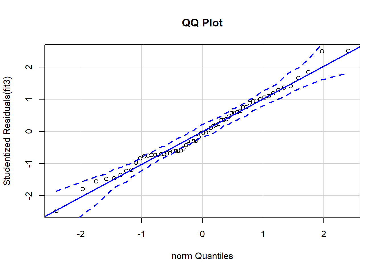
## 48 2.5026 0.015169 0.94046We have already used the qq normal plot of residuals in many places. We should not forget that it is a diagnostic tool and thus properly included in this chapter.
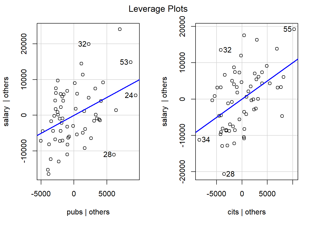
 The leverage plots shown here appear to be identical to the added variable plots shown above, and they are. The illustration here is done as a placeholder for later analyses where some IVs (such as categorical IVs with more than two levels) would have more than 1 df. In that case, this plot is useful, in addition to added variable plots.
A method of choice for addressing any violations of assumptions is often simple scale transformation of either the DV or the IVs, or both. We covered this idea with the household water use data set. We will revisit the scale transformation topic again at a later point in the course and will introduce Tukey’s ladder of scales and Box-Cox transformation. Here a quick implementation of Box-Cox transformation capabilities is introduced. In this instance, the goal is to find an exponent to use to transform the DV to help produce normality and homoscedasticity of the residuals. The peak of the curve in the plot yields \(\lambda\), the scaling component.
# scale transformations of the DV and/or IVs can help alleviate the impact of many issues
#  #evaluate possible Box-Cox transformations (MASS package must be installed)
# look for the lambda at the log likelihood peak
#library(MASS)
boxcoxfit3 <- boxcox(fit3,plotit=T)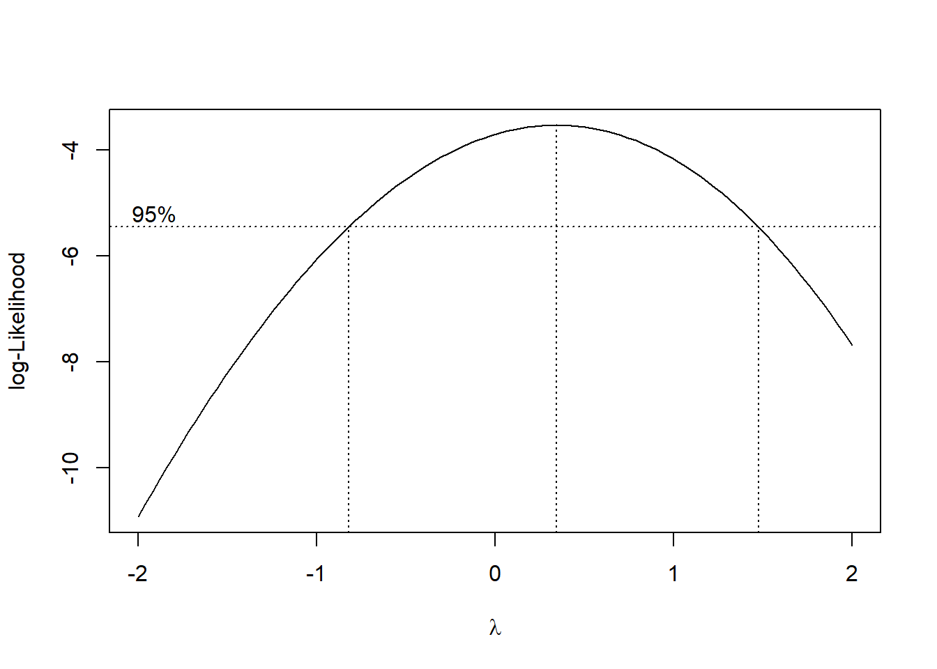
To find the exact \(\lambda\) value the output from the boxcox function was placed in a data frame and then sorted according to the log-likelihood value. The first case in the resorted dataframe gives the correct \(\lambda\) value. Note that the X and Y values are those used to create the plot above.
cox = data.frame(boxcoxfit3$x, boxcoxfit3$y)            # Create a data frame with the results
#str(cox)
cox2 <- cox[with(cox, order(-cox$boxcoxfit3.y)),] # Order the new data frame by decreasing y
#str(cox2)
cox2[1,] # Display the lambda with the greatest log likelihood
## boxcoxfit3.x boxcoxfit3.y
## 59 0.3434343 -3.531357For this model, \(\lambda\) is was found to be about .343. This value would be used to transform the DV and the analysis rerun. But recall that the normality and homoscedasticity assumptions didn’t appear to be violated so this process would be unnecessary for the current data set. I show the code just to provide a template. Notice that an exponent of 1.0 would not be a scale change. The exponent of .343 is approximately equivalent to the cubed root. Also note that with the scale change, the values of the regression coefficients would become less readily interpretable.