Chapter 14 Efficiency in OLS analysis using the olsrr package
The olsrr package has a collection of functions that streamline many of the piecemeal approaches oulined in earlier chapters. It makes it simple to obtain extensive/detailed information at once, with user-friendly functions. Not all of the topics covered in earlier chapters are included (e.g., semi-partial correlations), but extensive capabilities are also included for model criticism.
14.1 A basic analysis
The initial use of the ols_regress function can replace the individual uses of summary, anova, and confint functions. The model fit here is the three-IV model examined in the “Extensions” chapter.
##                            Model Summary
## --------------------------------------------------------------------
## R                       0.708       RMSE                   7030.542
## R-Squared               0.501       Coef. Var                12.826
## Adj. R-Squared          0.475       MSE                49428516.393
## Pred R-Squared          0.420       MAE                    5317.619
## --------------------------------------------------------------------
##  RMSE: Root Mean Square Error
##  MSE: Mean Square Error
##  MAE: Mean Absolute Error
##
##                                    ANOVA
## ----------------------------------------------------------------------------
##                       Sum of
##                      Squares        DF      Mean Square      F         Sig.
## ----------------------------------------------------------------------------
## Regression    2879765872.603         3    959921957.534     19.42    0.0000
## Residual      2866853950.768        58     49428516.393
## Total         5746619823.371        61
## ----------------------------------------------------------------------------
##
##                                        Parameter Estimates
## -------------------------------------------------------------------------------------------------
##       model         Beta    Std. Error    Std. Beta      t        Sig         lower        upper
## -------------------------------------------------------------------------------------------------
## (Intercept)    38967.847      2394.308                 16.275    0.000    34175.118    43760.575
##        pubs       93.608        85.348        0.135     1.097    0.277      -77.235      264.451
##        cits      204.060        56.972        0.361     3.582    0.001       90.019      318.102
##  degree_yrs      874.461       283.895        0.385     3.080    0.003      306.184     1442.739
## -------------------------------------------------------------------------------------------------
14.2 Collinearity diagnostics
The ols_coll_diag function provides collinearity diagnostics:
## Tolerance and Variance Inflation Factor
## ---------------------------------------
##    Variables Tolerance      VIF
## 1       pubs 0.5672118 1.763010
## 2       cits 0.8466483 1.181128
## 3 degree_yrs 0.5494035 1.820156
##
##
## Eigenvalue and Condition Index
## ------------------------------
##   Eigenvalue Condition Index   intercept        pubs        cits   degree_yrs
## 1 3.55809347        1.000000 0.009810827 0.014093645 0.009215181 0.0110334455
## 2 0.25588579        3.728942 0.146119575 0.358711061 0.097741038 0.0590237875
## 3 0.10745243        5.754407 0.015671115 0.619788632 0.026076066 0.9299270069
## 4 0.07856832        6.729533 0.828398483 0.007406662 0.866967715 0.0000157601
14.3 Added-variable plots
We can also obtain added-variable plots. These depict the partial correlations of each IV with the DV, both adjusted for other IVs. Here, it can be seen that pubs has a weaker partial relationship and this reinforces the fact that it’s test in the 3-IV model was non-significant. Recall that the partial correlation can be obtained with the mrinfo2 function. Unfortunately, partial and semi-partial correlations are not provided with the otherwise extensive information coming from ols_regress.
## `geom_smooth()` using formula 'y ~ x'
## `geom_smooth()` using formula 'y ~ x'
## `geom_smooth()` using formula 'y ~ x'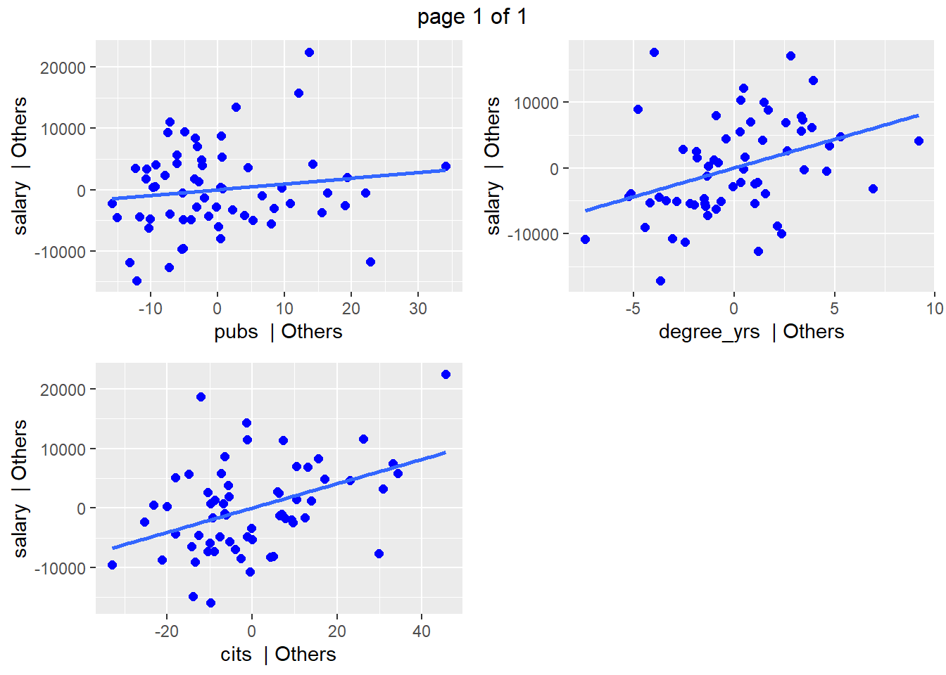
## [[1]]
## NULL
##
## $`supplemental information`
##            beta wt structure r partial r semipartial r tolerances  unique
## pubs       0.13506     0.71500   0.14254       0.10172    0.56721 0.01035
## cits       0.36102     0.77662   0.42559       0.33219    0.84665 0.11035
## degree_yrs 0.38541     0.85873   0.37495       0.28567    0.54940 0.08161
##             common   total
## pubs       0.24584 0.25618
## cits       0.19190 0.30224
## degree_yrs 0.28793 0.36954
##
## $`var infl factors from HH:vif`
##       pubs       cits degree_yrs
##   1.763010   1.181128   1.820156
##
## [[4]]
## NULL
14.4 Residual Assumptions
A normal QQ plot of the residuals is available.
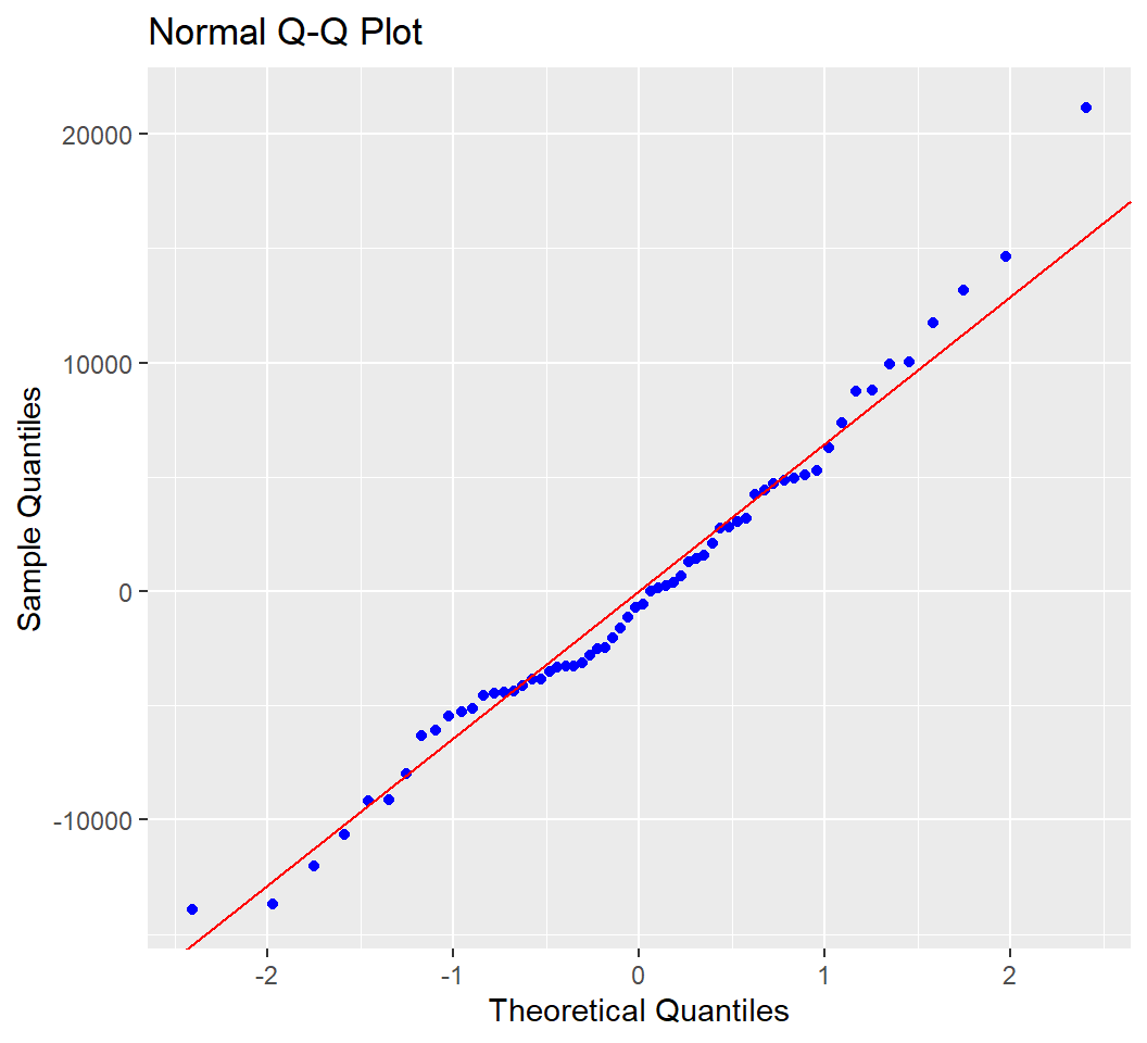
Tests of the residual normality assumption are easily obtained.
## -----------------------------------------------
## Test Statistic pvalue
## -----------------------------------------------
## Shapiro-Wilk 0.9782 0.3374
## Kolmogorov-Smirnov 0.0759 0.8404
## Cramer-von Mises 5.2312 0.0000
## Anderson-Darling 0.4327 0.2946
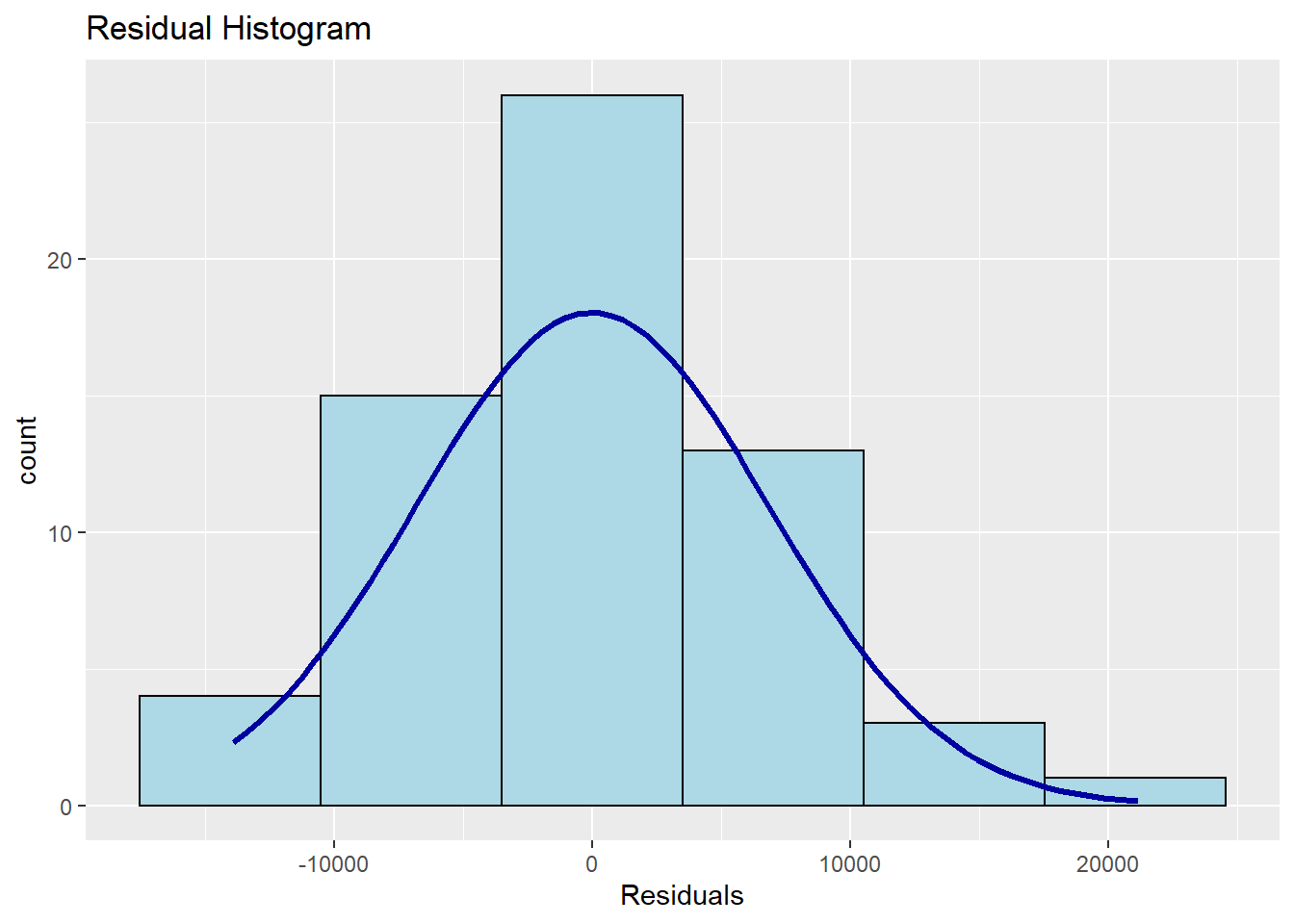
## -----------------------------------------------A histogram of the residuals with a normal curve overlaid for comparison is also available.
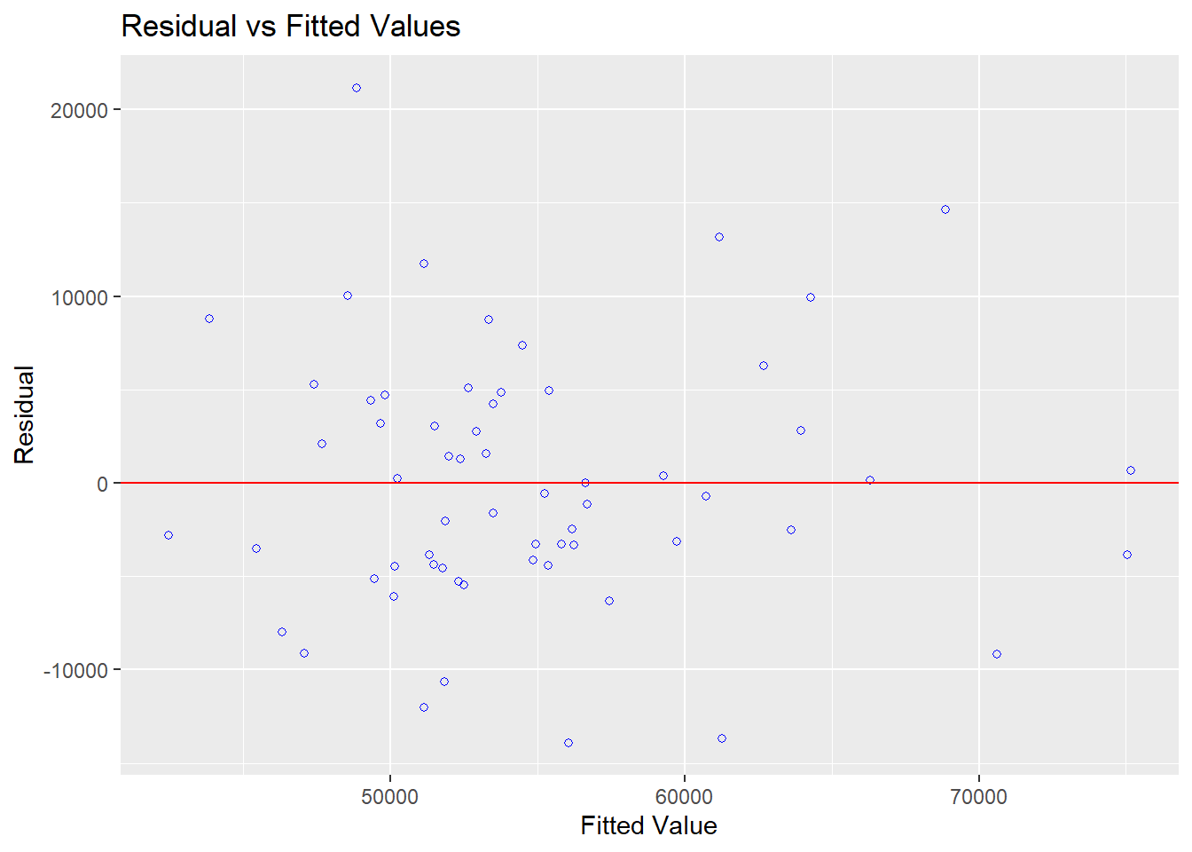
And the standard plot of residuals against yhats is also available.
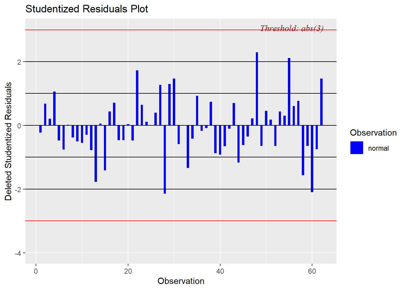
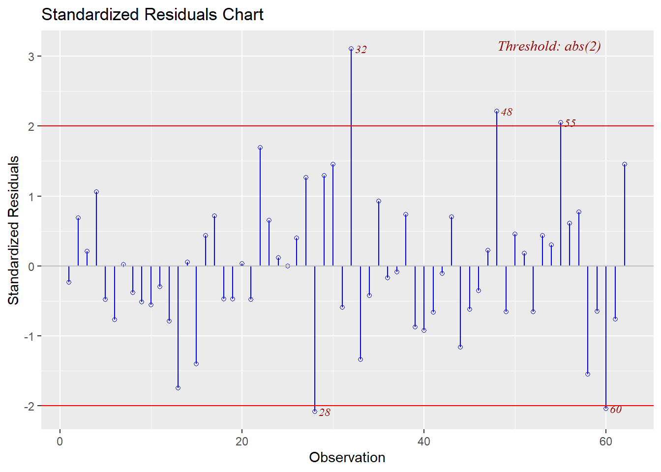
Studentized and Standardized residuals can be examined to look for sequential ordering effects in the data set by plotting them against the case number.
Several of the above plots plus other model diagnostic plots can be obtained more rapidly with the ols_plot_diagnostics function for which the code is shown here. The plots are not returned in order to save space.
14.5 Plots for examination of Influence
Several plots are available for visualizing the influence statistics for a model.
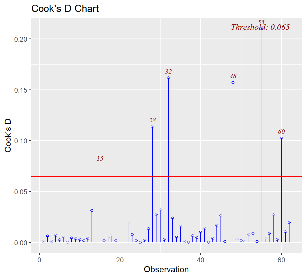
First is examination of Cook’s D values. It provides a visual indicators of which cases exceed a threshold for large influence and those cases are numerically labeled. I have not yet sorted out how this threshold is determined for this function and the following ones.
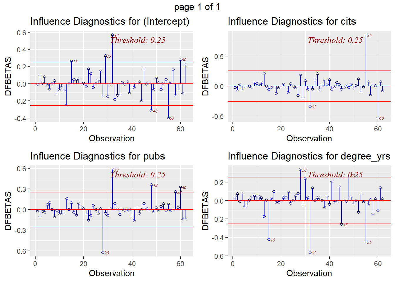
The DFBeta index is visualized with a panel of graphs, one for each IV and one for the intercept, permitting identification of influential cases for each IV separately.
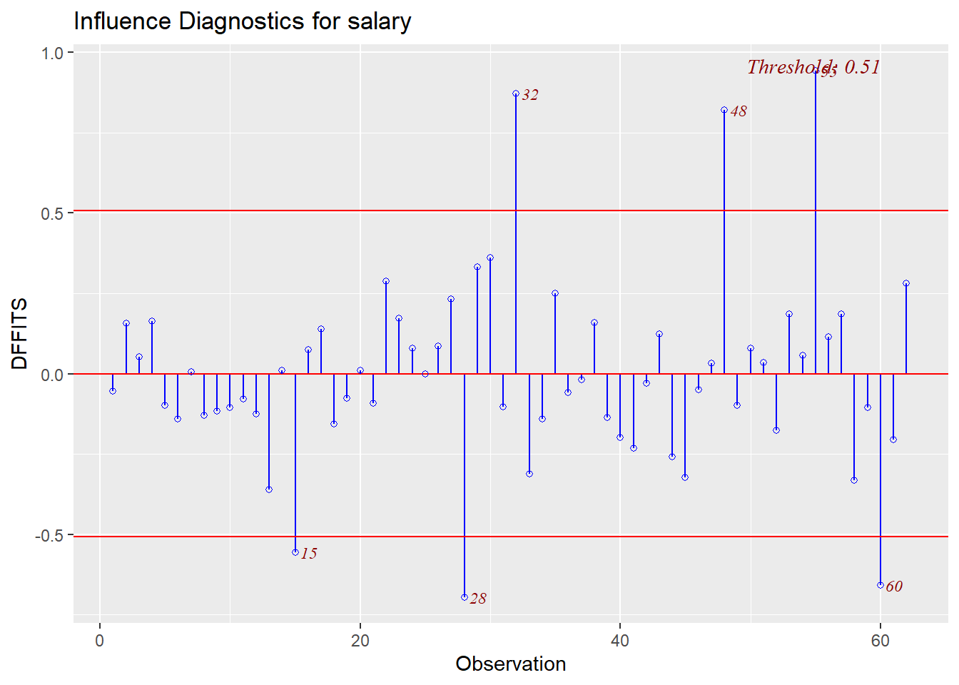
And a comparable plot for DFfits is also avaialble.
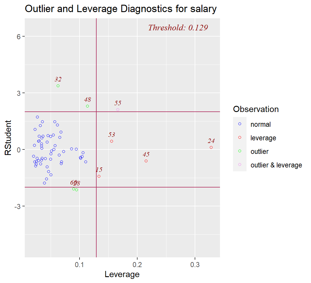
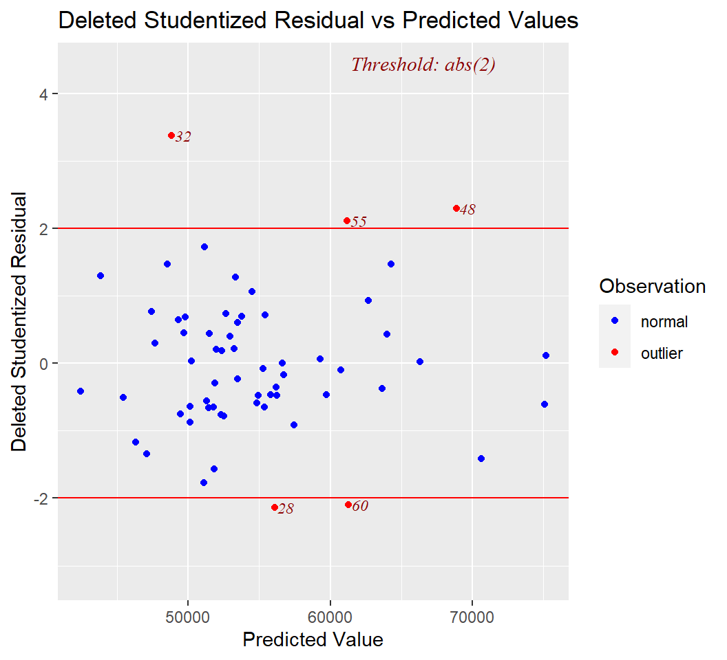
Finally, two additional plots are common in model diagnostics. They examine studentized residuals and deleted studentized residuals against leverage and yhats, respectively.
The **olsrr* package has numerous other tools and is worth exploring. The reference manual and vignettes on the CRAN site are very helpful.