Chapter 9 Inferential tests for assumptions

There are three primary assumptions that linear modeling with the standard NHST t and F tests rely on:

The relationships among variables are best described by linear functions.
The residuals from a model are normally distributed.
Homoscedasticity.

Graphical evaluation of these assumptions has been the priority in previous considerations, as well in this document. Now we can turn to inferential tests regarding these assumptions.

9.1 Evaluation of the Residual Normality Assumption

Prior work with SPSS and R for linear models has only employed a graphical assessment to the normality assumption for residuals (and skewness/kurtosis computation). Frequency histograms and normal probability plots are useful, but at times one may wish to do an inferential test of a null hypothesis that residuals are normally distributed. Quite a few such inferential tests have been developed, and many are available in R.

While we can easily accomplish these tests, the analyst should be concerned about a binary outcome decision process in evaluation of the assumption. The real question should be something like “with the degree of non-normality present, how much of an impact on the tests of regression coefficients and the test of the whole model is there?” Strong guidance on this is lacking. However, some discussion can be found in standard regression textbooks and the reader is advised to consult Fox (2016), or any number of other sources (e.g., Cohen et al. (2003), Cook & Weisberg (1999), Darlington (1990), Howell (2013), Weisberg (2014), or Wright & London (2009)).

The options available in R will be presented here without regard to that more important question. The Anderson-Darling test may be the test that is most recommended. Historically, the Shapiro test is probably the most commonly used one, based on availability in other software. But with the ‘nortest’ package in R, many others are also available.

First, we can implement the historically common Shapiro-Wilk test:

shapiro.test(residuals(fit3))

## 
## 	Shapiro-Wilk normality test
## 
## data:  residuals(fit3)
## W = 0.98639, p-value = 0.7239

This next code chunk shows code executing five different tests from the nortest package. But only one (Anderson-Darling) is executed here to keep this document small. The reader may recall from graphical approaches accomplished above that there is a slight degree of non-normality in the residuals from the basic two-IV model (fit3 or fit4). Is it a significant departure from normality, based on the sample size employed in this study?

# tests for normality of the residuals
#library(nortest)
ad.test(residuals(fit3)) # Anderson-Darling test (from 'nortest' package )

## 
## 	Anderson-Darling normality test
## 
## data:  residuals(fit3)
## A = 0.34507, p-value = 0.4742

#cvm.test(residuals(fit3)) #Cramer-von Mises test ((from 'nortest' package )
#lillie.test(residuals(fit3)) #Lilliefors (Kolmogorov-Smirnov) test (from 'nortest' package )
#pearson.test(residuals(fit3)) #get Pearson chi-square test (from 'nortest' package )
#sf.test(residuals(fit3)) #get Shapiro-Francia test (from 'nortest' package )

Neither of these tests reach significance thresholds at \(\alpha\)=.05 and this is not suprising given the small amount of skewness visualized in the graphical assessments of the residuals seen in above sections of this document.

9.1.1 Evaluation of the normality assumption by testing skewness and kurtosis

Another approach to inference regarding the normality assumption is to test whether skewness and/or kurtosis of the residuals deviates from a null hypothesis that they are zero (as would be the case for a normal distribution). Once again, this document is more concerned with showing how such tests can be accomplished in R. Discussions about their interpretation and whether they should be used are left to other parts of the course and to the recommendations of the relevant textbooks.

R has two packages (tseries and moments) that contain functions to test skewness and/or kurtosis:

# also....... another way to evaluate normality is to test for skewness and kurtosis
#library(tseries)
jarque.bera.test(residuals(fit3)) # Jarque Bera test for normality of a variable

## 
## 	Jarque Bera Test
## 
## data:  residuals(fit3)
## X-squared = 0.77247, df = 2, p-value = 0.6796

#library(moments)
agostino.test(residuals(fit3))

## 
## 	D'Agostino skewness test
## 
## data:  residuals(fit3)
## skew = 0.22341, z = 0.78060, p-value = 0.435
## alternative hypothesis: data have a skewness

anscombe.test(residuals(fit3)) # Anscombe-Glynn test of kurtosis

## 
## 	Anscombe-Glynn kurtosis test
## 
## data:  residuals(fit3)
## kurt = 2.68478, z = -0.25858, p-value = 0.796
## alternative hypothesis: kurtosis is not equal to 3

Again, none of these tests would allow us to reject a null hypothesis of residual normality.

We might also simply perform a Z test by taking the ratio of skewness and kurtosis coefficients to their std errors (called a large-sample approximation in using the std normal Z here). We can obtain the coefficients and std errors in a couple ways:

We can write our own function to test skewness and kurtosis as the Z approximation called the large sample approximation suggested above. First, create the function and test skewness:

# we can build our own tests, since we know the 
# std errors of skewness and kurtosis (fall semester work)
# these functions test the G1 and G2 statistics with their
# large sample std errors against nulls that the parameters are zero (as in normal distribs)
skewness.test <- function (lmfit) {
  require(psych)
  G1 <- psych::describe(residuals(lmfit),type=2)$skew # pull G1 from psych:::describe
  skewness <- G1
  N <- length(residuals(lmfit))
  stderrskew <- sqrt(6/N)
  teststat <- skewness/stderrskew
  pvalue <- 2*(pnorm(abs(teststat), lower.tail=F))
  outskew <- data.frame(cbind(N,G1,stderrskew,teststat,pvalue))
  colnames(outskew) <- c("N","G1","Std Error", "Z Test Stat","2-tailed p")
  rownames(outskew) <- c("")
  return(outskew)
}

# use this approach (z test) with large N. It returns a two-tailed p value 
skewness.test(fit3)

##   N        G1 Std Error Z Test Stat 2-tailed p
##  62 0.2289903 0.3110855   0.7361008  0.4616693

And now test kurtosis:

# now kurtosis
kurtosis.test <- function(lmfit) {
  require(psych)
  G2 <- psych::describe(residuals(lmfit),type=2)$kurtosis # pull G2 from psych:::describe
  kurtosis <- G2
  N <- length(residuals(lmfit))
  stderrkurt <- sqrt(24/N)
  teststat <- kurtosis/stderrkurt
  pvalue <- 2*(pnorm(abs(teststat), lower.tail=F))
  outk <- data.frame(cbind(N,G2,stderrkurt,teststat,pvalue))
  colnames(outk) <- c("N","G2","Std Error", "Z Test Stat","2-tailed p")
  rownames(outk) <- c("")
  return(outk)
}

kurtosis.test(fit3) # use this approach (z test) with large N. It returns a two-tailed p value

##   N         G2 Std Error Z Test Stat 2-tailed p
##  62 -0.2388151  0.622171  -0.3838415  0.7010959

9.2 Inferential test of Homoscedasticity

Evaluation of homoscedasticity shares the same graphical-approach history in our prior work as the normality assumption discussed above. There is also the question of relative impact of varying decrees of violation of the assumption that needs to be considered (we have discussed this previously in the context of the 2-sample location test assumption of homogeneity of variance which is essentially the same assumption). But the narrow goal here is the illustration of approaches in R. First, we redo a plot of residuals against yhats using the spreadLevelPlot function from the car package. The plot gives a hint of larger residual spread for mid range values of yhats, but the pattern is carried by only a few data points.

# also a plot slightly different from the base system plot on the fit
# from the car package
spreadLevelPlot(fit3)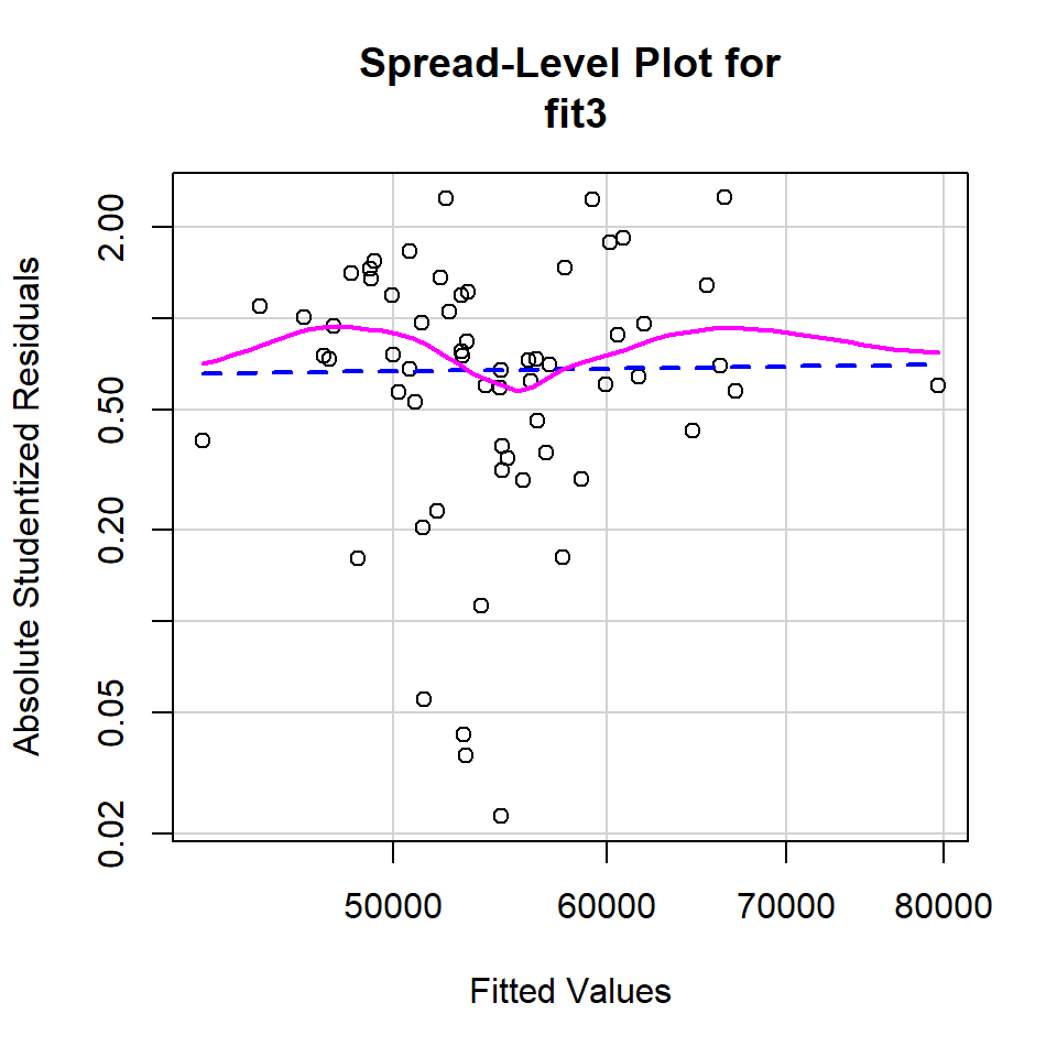

## 
## Suggested power transformation:  0.8964362

The ncvTest function (ncv standing for non-constant variance), also from the car package provides chi-square based test statistic that evaluates a null hypothesis of homoscedasticity. The test is more typically called the “Score” test.

# tests of homoscedasticity
# the ncvTest function is a test of non-constant error variance, called the Score test from car
ncvTest(fit3)

## Non-constant Variance Score Test 
## Variance formula: ~ fitted.values 
## Chisquare = 0.2914146, Df = 1, p = 0.58932

Another test of homoscedasticity is one that is frequently used. The Breusch-Pagan test is implemented in the bptest function found in the lmtest package. Neither it, nor the Score test yielded a result that would challenge the null hypothesis of homoscedasticity.

#library(lmtest)
bptest(fit3)

## 
## 	studentized Breusch-Pagan test
## 
## data:  fit3
## BP = 2.665, df = 2, p-value = 0.2638

9.3 Global Evaluation of Linear Model Assumptiions using the ‘gvlma’ package.

A recent paper in JASA (Pena & Slate, 2006) outlined an approach to model assumption evaluation that is novel (and mathematically challenging). An R implementation is now available in the gvlma package. Initially, the approach evaluates a global null hypothesis that all assumptions of the linear model hypothesis tests are satisfied:

Linearity
Normality evaluation of skewness)
Normality (evaluation of kurtosis)
Link Function (linearity and normality)
Homoscedasticity

If this global null is rejected, then evaluation of each of four component assumptions is evaluated individually.

Fortunately, the ‘gvlma’ function is simple to use and the output is largely the standard NHST p value for each test.

A caveat here is that this type of approach is even more likely to be the target of the kinds of discussion we have had before on whether binary decision inferential tests are the way to act on knowledge of whether model assumptions are satisfied. I have not yet found a literature commenting on or assessing the Pena & Slate procedure (2006), so use of this method is only recommended with reservation. It does serve as a good example of how new/novel methods become rapidly available in R and are sometimes quite simple to implement.

# both the package and the function are called 'gvlma'
#library(gvlma)
# the gvlma function only requires a 'lm' model fit object as a single argument to yield the full assessment
gvlmafit3 <- gvlma(fit3)
#print out the tests
gvlmafit3

## 
## Call:
## lm(formula = salary ~ pubs + cits, data = cohen1)
## 
## Coefficients:
## (Intercept)         pubs         cits  
##     40493.0        251.8        242.3  
## 
## 
## ASSESSMENT OF THE LINEAR MODEL ASSUMPTIONS
## USING THE GLOBAL TEST ON 4 DEGREES-OF-FREEDOM:
## Level of Significance =  0.05 
## 
## Call:
##  gvlma(x = fit3) 
## 
##                     Value p-value                Decision
## Global Stat        1.8686  0.7599 Assumptions acceptable.
## Skewness           0.5158  0.4727 Assumptions acceptable.
## Kurtosis           0.2567  0.6124 Assumptions acceptable.
## Link Function      0.2047  0.6509 Assumptions acceptable.
## Heteroscedasticity 0.8914  0.3451 Assumptions acceptable.

#plot relevant information
# note: this plot does not play nice in the R markdown format.  
#       So I generated it outside of the .Rmd file, saved the image and displayed the image below
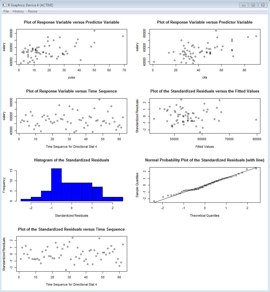
#plot(gvlmafit3)

It is possible to generate a set of very useful plots by passing the gvlma object just created to the base system plot function (plot(gvlmafit3) as was commented out in the code chunk just above). However, the figure doesn’t play nice with rmarkdown, so I created it separately, and saved the figure to a .png file that is displayed here.