Chapter 5 Review Unique and common proportions of variance and Type I vs III Sums of Squares
We can think about an ability to partition the SS of the DV, not only into Regression and Residual components, but to further break down the Regression SS into unique and common parts. This builds on the concepts just reviewed above and connects to earlier work.
THIS SECTION AND THE NEXT ARE THE CRITICAL CONCEPTUAL FRAMEWORK THAT HAS BEEN DEVELOPED FOR MULTIPLE REGRESSION IN THE 510/511 COURSE. WE COVERD THIS WHEN WE WORKED THROUGH THE SPSS IMPLEMENTATION. IF YOU DID NOT CONSOLIDATE IT THEN, OR ON ASSIGNMENTS/EXAM PREP, THEN THIS IS THE TIME/PLACE TO BE CERTAIN ABOUT IT.
In this section we will: 1. find unique SS for each IV, and the common SS 2. Utilize semi-partial correlations and the derived unique/common proportions from ‘mrinfo’ 3. use these quantities to reinforce concepts that we have repeatedly covered in slightly different ways 4. use R as a calculator to accomplish some of these things 5. Understand that since we are going to use some rounded quantities from ‘mrinfo’ some error is introduced into our computations. So, some things may not match exactly as the should if the concepts are correct.
5.1 SS components, semi-partial correlations, unique and common proportions/SS
A few components are computed “manually” to establish some basic quantities. SStotal is found two different ways (the quantities are returned after this code chunk), and they match. Other quantities are calculated, but not printed here - they are used below.
# compute a few SS manually.....
# first obtain a few values to use, SS Total, MSresid, and R squared
SStotal <- var(cohen1$salary)*61 # variance times n-1 gives SS for that variable
# name an object that is the anova summary table for the fit3 model
a <- anova(fit3)
#extract the MS Residual and multiple R squared from that table
MSresid <- a$`Mean Sq`[3]
rsquared <- summary(fit3)$r.squared
# use the above quantities to compute SS Regression and SS Residual
SSregression <- rsquared*SStotal
SSresidual <- MSresid*59 # MS resid times its df
# sum them to doublecheck
SSregression + SSresidual # should equal SStotal
## [1] 5746619823## [1] 5746619823Focus on the information value of the semi-partial correlations (we found them with mrinfo above). By squaring them, we have the unique proportions of variance accounted for by each IV - and the values match what was reported by mrinfo above.
semipartialpub <- .3424509
semipartialcit <- .4041425
# square them to produce "unique" proportions of explained variance
# see that it matches the table from mrinfo
part1sqrd <- semipartialpub^2
part2sqrd <- semipartialcit^2
part1sqrd
## [1] 0.1172726## [1] 0.1633312Now, we can use the squared semi-partials to find the common proportion of variance shared between the two IVs. Does it match what was returned by mrinfo?
# now that we know the unique fractions we can find the common proportion
# and it should match the mrinfo value
# recall that rsquared was defined at the beginning of this section
commonprop <- rsquared -part1sqrd - part2sqrd
commonprop
## [1] 0.138912Now compute the unique and common SS. It would be useful to compare these SS to the table found above in the basic model section for fit3 and fit4 and the section that compared the ANOVA summary tables from anova and Anova.
# now compute the unique and common SS
uniqueSSpub <- part1sqrd*SStotal
uniqueSScit <- part2sqrd*SStotal
uniqueSSpub
## [1] 673921157## [1] 938602084These do match the SS for the two IVs found by using the Anova function (with type III SS) from either fit3 or fit4. What is their sum? It should be less than SS regression since each is the unique component and the full SSregression includes the common SS where the two IVs overlap in the salary space.
# should these two values add up to SSregression?
# No.   should be something less
uniqueSSpub + uniqueSScit
## [1] 1612523240## [1] 2410797436Lets find a common SS by using the common proportion seen above.
# how much less??????? the amount due to the shared SS
# its proportion is the common proportion
commonprop
## [1] 0.138912## [1] 798274196Now verify that all three components sum to SSregression, as they should:
## [1] 2410797436## [1] 24107974365.2 F tests on the unique components?
Now that we have derived unique SS for each IV, can we do an F test? That is, can we test a null hypothesis that an individual IV does not uniquely contribute to the R squared (also phrased as the model fit)? Yes. Just like any F test:
First, find the MS for each IV, based on the unique SS.
# can we do tests of these unique SS? Sure, F tests with MSresid as "error" term
# We need to convert the unique SS to MS, so we need df
# each has 1 df, since each represents one variable
# the MS are the SS divided by 1
MSuniquepub <- uniqueSSpub/1
MSuniquecit <- uniqueSScit/1
MSuniquepub
## [1] 673921157## [1] 938602084Now find the F values by using MSresid as established above.
# and now the two F's
Fpubunique <- MSuniquepub/MSresid  #(df are 1,59)
Fcitunique <- MSuniquecit/MSresid  #(df are 1,59)
Fpubunique
## [1] 11.9195## [1] 16.60086# can you find these F's anywhere above?
# hint: look in the table of the Anova function (not anova)Yes, they match the F’s from the Anova tables above, using Type III SS. And, we can take their square roots to compare to the t values for each regression coefficient. This duplicates the illustration seen in a previous chapter.
## [1] 3.452463## [1] 4.074415# look familiar???
# yes, they are the t's that provided the test stat for the regression coefficientsConclusions?
- tests of semipartial correlations can be done as F tests by converting to SS and MS
- these tests are equivalent to the F tests done on TYPE III SS in the Anova function
- since the F’s are the squares of the t’s for the two regression coefficients, we conclude that tests of the regression coefficients are tantamount to tests of the semi-partial correlations. This is why we can call them partial (actually semi-partial) regression coefficients.
- The unique SS are seen to be equivalent to the SS computed above by the ‘Anova’ function (rather than ‘anova’), and are thus equivalent to what are called Type III SS. To be contained……
5.3 Compare and Contrast information from fit3 and fit4
Take some time again to ponder the output from above, comparing comparable values from fit3 and fit4 as we did in the previous chapter. Recall that fit3 and fit4 differed only in the order of entry of the two IVs, with pubs first in fit3. Many/most of the components are the same. The primary differences seem to emerge in the ‘anova’ vs ‘Anova’ output. Take the square root of each of the F tests from ‘anova’ and ‘Anova’. Which ones match the t’s for tests of the comparable regression coefficients and which differ? This was explored briefly earlier in this document. This section reviews that information again in a more succinct tablular form. I have created a table of SS produced by both ‘anova’ and ‘Anova’ for each of fits 3 and 4 to facilitate this comparison. Make certain you can see, in the above output, where these values came from.
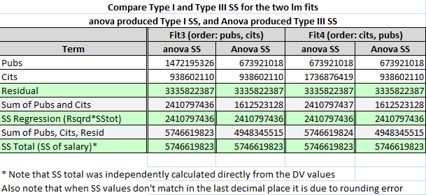
For the moment, notice a few things from this table, recalling that both fit3 and fit4 have the same intercept, regression coefficients and their t’s, multiple R squared, SS total, SS residual, SS regression, and F-tests of the whole equation with 2 and 59 df. The SS for pubs and cits should be a partitioning of SS regression.
- In ‘anova’ output, the sum of the SS for pubs and cits matches SS regression both for fit3, and fit4 which also match each other.
- In ‘Anova’ output the sum of the SS for pubs and cits is always less than SS Regression, and adding them to SS residual yields a quantity less that SS total.
- For ‘anova’ output, summing SS for pubs, cits, and residual DOES yield the SS total, as expected.
- Sometimes SS for pubs (or for cits) from ‘anova’ and ‘Anova’ match and sometimes they don’t. It depends on which fit one examines. So, we must conclude that the ‘order’ of model specification has something to do with the difference in Type I and Type III SS. Type III SS are found by treating each IV as if it were the last to enter the model, thus controlling for all other IVs.
- The reader might also compare the SS for each IV under each model to the SS Regression from when that IV was used in simple regression in this document (in the bivariate computations section)
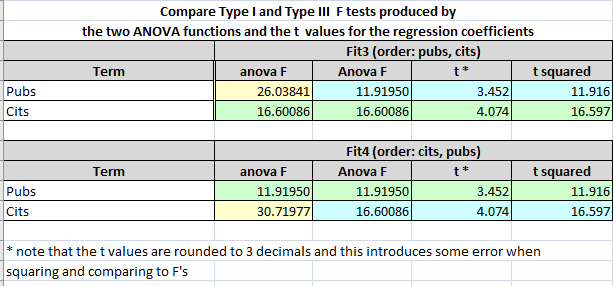
A similar table compares F test values from ‘anova’ and ‘Anova’ for the two fits. The pattern here follows what was seen for SS above since the F’s are derived from those SS. The more interesting comparison is the comparison of those F’s to the square of the t’s found from testing the two regression coefficients in the two models. This comparison lets us get to the heart of what is being tested with the F tests vis a vis the way we discussed the null hypotheses for the t tests of the regression coefficients.
The t’s test a null hypothesis that the “unique” contribution of that predictor is zero, when controlling for the other predictor(s). And the squares of these t’s don’t always match the F’s from the ‘anova’ function. They do match for the ‘Anova’ function. Further discussion of this took place above, connecting the findings to concepts deriving from our understanding of semi-partial correlations.
This general topic is further addressed below entitled “Work with Sums of Squares a bit more, along with unique and common proportions of variance.”
Typically we would not evaluate both models fit3 and fit4 which entered the IVs in different orders since to final model is largely the same (with the caveat about unique vs sequential or Type I vs Type III SS). If you examined the coefficients tables for fit3 and fit4, you found the regression coefficients to be the same (and the t-tests of them as well) So much of the above work is duplicative. Perhaps we would only run fit3. In that case, the kind of comparison in the next section on formally comparing models might still be of interest.
The issue with types of SS computation is revealing in this comparison of fit3 and fit 4 which have only two IVs. The SS computation issue will be addressed several times later in the semester and becomes more involved when the number of IVs exceed two. For now, focus on the comparability of the fit3 and fit4 models with regard to overall fit, and with regard to coefficients. Additional illumination on fit3 and fit4 differences in SS will be connected to semi-partial correlations and unique vs common SS issues addressed below and that is the part of this topic that is the important conceptual framework. The primary conclusion from the SS comparison work here, is that order of entry of the IVs into a model can affect the SS computation, depending on whether the analyst chooses Type I (sequential) or Type III (unique) SS.