Chapter 7 Further work with residuals and yhats

This section is structured with three goals:

Learning how to extract the residuals and the yhats from a ‘lm’ fit object in order to do additional work with them. You may recall that we learned to “save” residuals and yhats from an SPSS regression. That is also done here.
The diagnostic plots from above did not give us a frequency histogram of the residuals or even a simple boxplot. Once extracted, we can easily produce those types of graphs.
We can revisit some primary concepts in linear modeling by further examining the meaning of the yhats.

First, extract the residuals and yhats from the model fit (fit3 in this instance). We could add them to the data frame containing the original variables for later potential use (although we can work with the newly created vectors directly here.

fit3.resid <- residuals(fit3)
fit3.pred <- predict(fit3)
#create a new data frame with the original variables plus the exracted residuals and yhats
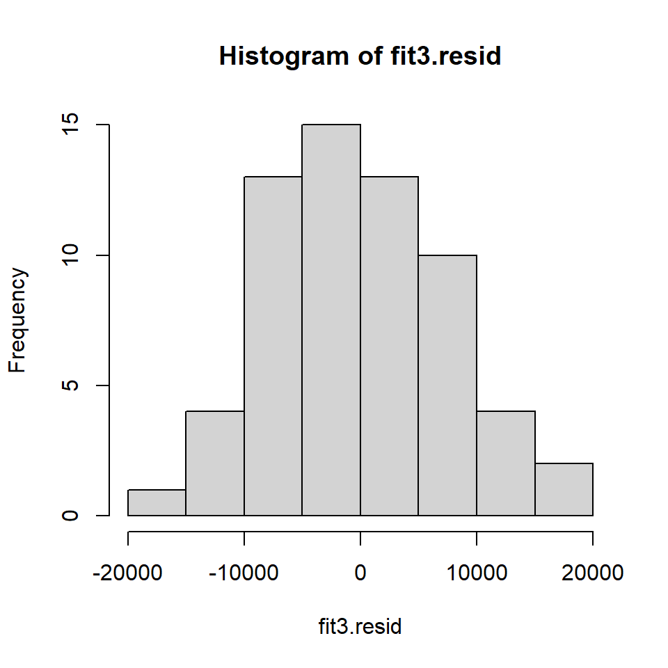
cohen2 <- cbind(cohen1,fit3.resid,fit3.pred) #note that fit3.pred is the yhats

Examine the frequency histogram of the residuals. It looks only slightly positively skewed even though the original DV was somewhat skewed. The normality assumption may not be seriously violated.

# simple frequency histogram of the residuals from fit3
hist(fit3.resid)

Boxplots of the residuals and yhats are produced next, revealing one potential outlier in the yhats.

# boxplots
layout(matrix(c(1,2),1,2)) #optional 2graphs/page 
boxplot(fit3.resid,xlab="Residuals",data=cohen2,col="lightgrey")
boxplot(fit3.pred, xlab="Yhat",data=cohen2,col="lightgrey")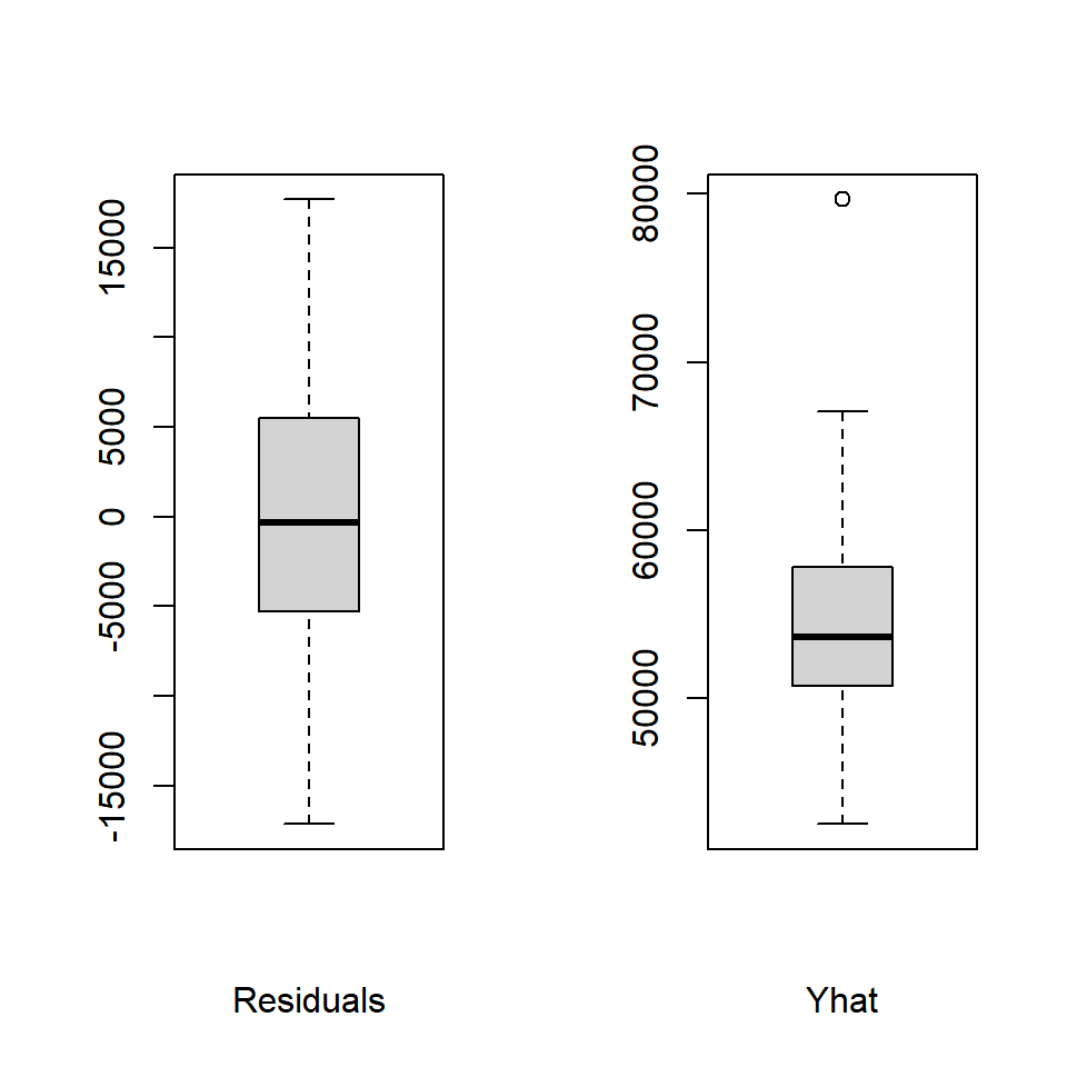

Numerical summaries of the residuals and yhats are provided by the describe function.

psych::describe(fit3.resid)

##    vars  n mean      sd  median trimmed     mad       min      max    range
## X1    1 62    0 7394.97 -341.27 -160.91 7519.46 -17133.14 17670.34 34803.48
##    skew kurtosis     se
## X1 0.22     -0.4 939.16

psych::describe(fit3.pred)

##    vars  n     mean      sd   median  trimmed     mad      min      max range
## X1    1 62 54815.76 6286.59 53630.77 54275.57 4982.75 42497.52 79670.52 37173
##    skew kurtosis    se
## X1 1.13     2.45 798.4

Now that we have the yhat values available, we can do one more analysis that will be familiar. If we correlate the yhats with salary (the DV), we find an interesting quantity, when we square it.

# correlate the original DV (salary) with the yhats from the two-IV linear model 
r_y_yhat <- with(cohen2, cor(salary, fit3.pred))
r_y_yhat

## [1] 0.6477003

# square that value
r_y_yhat^2 #does the value look like something you recognize?

## [1] 0.4195157

When covering this characteristic at earlier points, it was emphasized that the yhats are the best linear combination of the IVs, and carry all the information about the predictability of the DV from those IVs. It is a core feature of regression that the relationship between the DV and the yhats reveals the strength of the prediciton, the multiple R (or R-squared).